How to do hyperparameter tuning using Azure ML
Created:
Updated:
Topic: Azure ML: from beginner to pro
Introduction
When training a machine learning model, choosing the right values for your hyperparameters (such as learning rate) makes a world of difference in the quality of the model’s predictions. You can start to get a feel for which hyperparameter values work best by trying a few values manually, but automating this search is key to achieving the best results. There are several packages that can help you automate this search — for example, when I’m working on projects that use PyTorch and not Azure ML, I often rely on Ray Tune. But when I’m developing a project that uses Azure ML to train in the cloud, I prefer to use an Azure ML Sweep Job for hyperparameter tuning. I especially love how simple my code looks when I use a Sweep Job — I can write the code assuming that the hyperparameter values are passed as arguments, and specify all the parameter search logic in an easy-to-read YAML file. Read on to find out how!
I assume that you already have a good understanding of what hyperparameter tuning is, and that you know how to train a model in Azure ML — if you need a refresher, check out my blog post on the topic.
The project that illustrates the topics in this post can be found on GitHub. The README file for the project contains details about Azure and project setup.
Training and inference on your development machine
It’s always a good idea to run your ML training code on your development machine before bringing it to the cloud. You can do that by clicking “Run and Debug” in VS Code’s left navigation, selecting the “Train locally” run configuration, and pressing F5. This code uses the Fashion MNIST dataset to train a simple neural network, and it generates two directories: data to which it downloads Fashion MNIST data, and model to which it saves the trained model.
To keep this sample straightforward, I chose only two hyperparameters to tune: learning rate and batch size. In a real-world scenario, you probably want to identify many more hyperparameters, such as the settings for your optimizer and any other values that feel like a guess. I add each hyperparameter as an argument in my code, and I give them default values, as you can see in train.py:
def main() -> None:
    logging.basicConfig(level=logging.INFO)

    parser = argparse.ArgumentParser()
    ...
    parser.add_argument("--learning_rate",
                        dest="learning_rate",
                        default=0.001,
                        type=float)
    parser.add_argument("--batch_size", dest="batch_size", default=64, type=int)
    ...
    args = parser.parse_args()
    ...
Since the model was saved using MLflow, you can take a look at the values logged during training using the MLflow UI, with the following command:
mlflow ui
Open your browser to the link shown in the output of the command, then click on metrics. You should see a validation accuracy of about 65%. We should be able to achieve a higher accuracy by tuning our hyperparameters.
You can also make a local prediction using the trained MLflow model. You can use either CSV or JSON files:
cd aml_sweep
mlflow models predict --model-uri "model" --input-path "test_data/images.csv" --content-type csv
mlflow models predict --model-uri "model" --input-path "test_data/images.json" --content-type json
Training and deploying in the cloud
Once we’ve determined that the training code works well on our development machine, we’re ready to execute it in the cloud. Our first steps are to create a CPU cluster which specifies the VMs we want to use for training, and a data resource which will make our data easily accessible in the cloud. If you followed my posts on basic training, creating a pipeline, or mixing resource creation methods, you already have these resources created in Azure ML, so you can skip this section.
Here’s cluster-cpu.yml, the YAML file that specifies the configuration for a cluster of 0-4 CPU VMs in Azure ML:
$schema: https://azuremlschemas.azureedge.net/latest/amlCompute.schema.json
name: cluster-cpu
type: amlcompute
size: Standard_DS4_v2
min_instances: 0
max_instances: 4
And here’s the CLI command to create the cluster from this configuration file:
az ml compute create -f cloud/cluster-cpu.yml
The data YAML file data.yml points to the location of the data folder on our development machine:
$schema: https://azuremlschemas.azureedge.net/latest/data.schema.json
name: data-fashion-mnist
description: Fashion MNIST Dataset.
path: ../data/
And here’s how we can bring that data to the cloud:
az ml data create -f cloud/data.yml
Now we have everything we need to create an Azure ML Job that trains our code in the cloud. If you’ve read my previous posts, you’ve seen how to create a CommandJob to do simple training, and how to create a PipelineJob to train in a sequence of steps. In this post we’ll create another type of job, called a SweepJob, to do hyperparameter tuning. When Azure ML executes a sweep job, it starts several trials, each with a different set of hyperparameter values. When all trials complete, it picks the one that gave us the best result. What does “best” mean in this case? It’s up to us — we get to define a measure that we want to maximize or minimize in the YAML file.
Let’s look at the complete sweep-job.yml file, which defines how we want hyperparameter tuning to be done. I’ll explain each setting in detail next.
$schema: https://azuremlschemas.azureedge.net/latest/sweepJob.schema.json

type: sweep
description: Trains a simple neural network on the Fashion-MNIST dataset.
compute: azureml:cluster-cpu

inputs:
  fashion_mnist:
    path: azureml:data-fashion-mnist@latest
outputs:
  model_dir:
    type: mlflow_model

search_space:
    learning_rate:
        type: loguniform
        min_value: -6.90775527898 # ln(0.001)
        max_value: -2.30258509299 # ln(0.1)
    batch_size:
        type: choice
        values: [32, 64, 128, 256]

trial:
  code: ../src
  command: >-
    python train.py
    --data_dir ${{inputs.fashion_mnist}}
    --learning_rate ${{search_space.learning_rate}}
    --batch_size ${{search_space.batch_size}}
    --model_dir ${{outputs.model_dir}}
  environment:
    image: mcr.microsoft.com/azureml/openmpi4.1.0-ubuntu20.04:latest
    conda_file: conda.yml

objective:
  goal: maximize
  primary_metric: validation_accuracy

sampling_algorithm:
  type: random

early_termination:
  type: median_stopping
  evaluation_interval: 1

limits:
  max_total_trials: 12
  max_concurrent_trials: 4
  timeout: 36000 # in seconds (10 hours)
  trial_timeout: 7200 # in seconds (2 hours)
The YAML file starts by specifying the schema for a sweep job, which lets VS Code provide Intellisense when we’re editing the file. We set type to sweep to indicate that this is a sweep job, and we set description to a short summary that will show up in the Azure ML Studio entry for this job. In the compute setting, we specify that we want training to run on the CPU compute cluster we created earlier.
$schema: https://azuremlschemas.azureedge.net/latest/sweepJob.schema.json

type: sweep
description: Trains a simple neural network on the Fashion-MNIST dataset.
compute: azureml:cluster-cpu
...
The YAML file specifies that our training job has one input argument (the data resource we created earlier) and one output argument (the folder that will contain the trained model). Notice that we can always get the latest version of our data by adding @latest to the end of the resource name. The default type for inputs is uri_folder, and our data is saved to a folder, so we don’t need to specify a type. Another common type for data is uri_file, in case our data was stored in a single file. Our output is a model saved using MLflow, so we need to specify its type to be mlflow_model. Another common type for models is custom_model, in case we hadn’t used MLflow to save it. You can press Ctrl+Space in the appropriate line within VS Code to get Intellisense help for the allowed types.
...
inputs:
  fashion_mnist:
    path: azureml:data-fashion-mnist@latest
outputs:
  model_dir:
    type: mlflow_model
...
The search_space section contains the names of the hyperparameters we want to tune, and information on how we want to tune them. Our first hyperparameter is learning_rate, and we want to consider values between 0.001 and 0.1. We’ll likely get better results if we consider values with more granularity at the lower end and less granularity at the upper end, so we use a loguniform distribution to sample them. Keep in mind that the min and max values you need to specify in the YAML are the natural logarithms of the actual min and max values you want — therefore, in this case we set the minimum value to ln(0.001), and the maximum value to ln(0.1). Our second hyperparameter is batch_size, and we want to consider only four different values, so we specify its type to be choice, and we give it a list with the values we want.
...
search_space:
    learning_rate:
        type: loguniform
        min_value: -6.90775527898 # ln(0.001)
        max_value: -2.30258509299 # ln(0.1)
    batch_size:
        type: choice
        values: [32, 64, 128, 256]
...
You can use Intellisense to see all types of search spaces supported:

These refer to names of common statistical functions, so you can easily find more information about each of them on the internet.
Under the trial section, we specify where our code is located and the command used to run it — notice how we use the special syntax ${{...}} to refer to the input, the output, and the hyperparameters defined in the search_space. My training code expects all of these as arguments. We also specify the software environment we want installed in the CPU cluster. You can learn more about how to choose a good environment in my blog post on the topic.
...
trial:
  code: ../src
  command: >-
    python train.py
    --data_dir ${{inputs.fashion_mnist}}
    --learning_rate ${{search_space.learning_rate}}
    --batch_size ${{search_space.batch_size}}
    --model_dir ${{outputs.model_dir}}
  environment:
    image: mcr.microsoft.com/azureml/openmpi4.1.0-ubuntu20.04:latest
    conda_file: conda.yml
...
In the objective section, we specify that our goal is to maximize the validation accuracy:
...
objective:
  goal: maximize
  primary_metric: validation_accuracy
...
The validation_accuracy metric is logged with that exact name in the training code in train.py:
def train(data_dir: str, learning_rate: float, batch_size: int, model_dir: str,
          device: str) -> None:
    """
    Trains the model for a number of epochs, and saves it.
    """
    ...
    for epoch in range(epochs):
        logging.info("Epoch %d", epoch + 1)
        (training_loss, training_accuracy) = fit(device, train_dataloader,
                                                 model, loss_fn, optimizer)
        (validation_loss,
         validation_accuracy) = evaluate(device, val_dataloader, model, loss_fn)

        metrics = {
            "training_loss": training_loss,
            "training_accuracy": training_accuracy,
            "validation_loss": validation_loss,
            "validation_accuracy": validation_accuracy
        }
        mlflow.log_metrics(metrics, step=epoch)
    ...
The sampling_algorithm section is where we specify how we want data to be sampled from the statistical functions we chose earlier. I opted to randomly sample values.
...
sampling_algorithm:
  type: random
...
You can use Intellisense to see the list of supported sampling algorithms:

You can find plenty of detailed information about each sampling algorithm on the internet, but here’s a quick summary:
- Bayesian - Values are sampled based on how previous samples performed when evaluated against the primary metric.
- Grid - Values are sampled in a grid over the specified search space.
- Random - Values are sampled randomly.
The early_termination section allows you to specify an algorithm that stops training when the performance of the primary metric starts to degrade.
...
early_termination:
  type: median_stopping
  evaluation_interval: 1
...
You can use Intellisense to see the list of supported early termination algorithms:

Here’s a quick summary of early termination algorithms supported by Azure ML:
- Bandit - Cancels a job when the primary metric isn’t within a specified slack factor.
- Median Stopping - Cancels a job based on the running average of its primary metric.
- Truncation Selection - Cancels a percentage of lowest performing jobs at each evaluation interval.
We can also specify certain limits for our trials. As you can see below, I instructed Azure ML to run a maximum of 12 trials (each with its own set of hyperparameter values), and no more than four concurrently. Why four? Recall that our CPU cluster was configured to support 0 to 4 VMs. If I have four concurrent trials going on at once, I’m maximizing the utilization of my cluster, and therefore getting results in an optimal amount of time. It doesn’t make much sense to choose a number of trials larger than the number of VMs in your cluster. But you could certainly choose a smaller number — this is a common scenario in fact, when you have other code running on the same cluster.
I also tell Azure ML to timeout the whole sweep run within 10 hours, and to timeout each trial within 2 hours. This may come in handy in case processing gets stuck for some reason.
...
limits:
  max_total_trials: 12
  max_concurrent_trials: 4
  timeout: 36000 # in seconds (10 hours)
  trial_timeout: 7200 # in seconds (2 hours)
...
You can look at the documentation to learn more about defining a sweep.
Now that we’ve discussed every line in the YAML file for the training job, we’re ready to run it in the cloud:
run_id=$(az ml job create -f cloud/sweep-job.yml --query name -o tsv)
This job will take a while, because it executes a maximum of 12 trials, each evaluating a different combination of hyperparameter values. You can follow along in the Studio, under “Jobs,” “aml_sweep,” then “Trials.”
Once the job is completed, the Trials section will display information and graphs from the 12 trials:
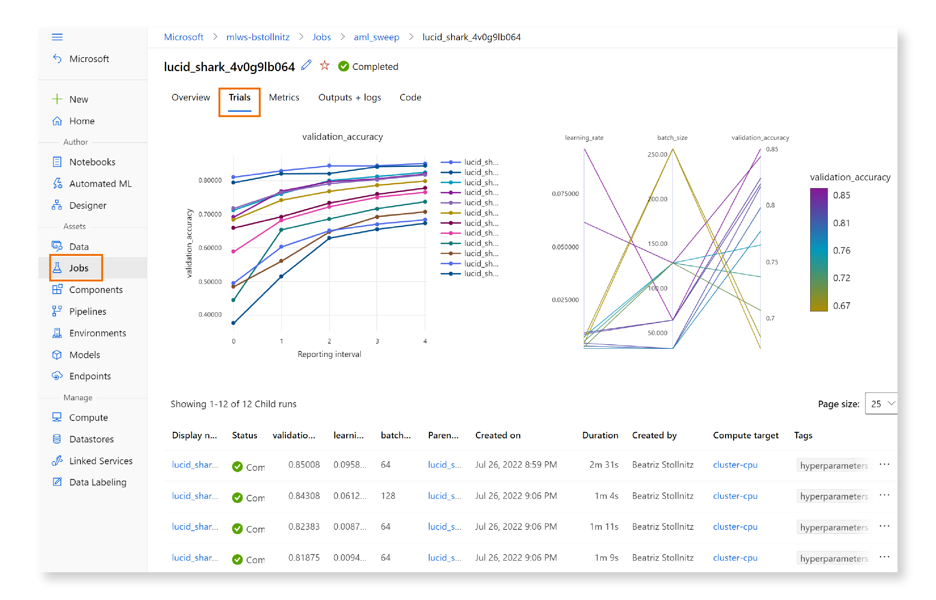
In the “Overview” section, look for “Primary metric,” and you’ll find a link to the trial that performed best according to our chosen metric.

If you click on that link, you’ll see that the best trial achieved a validation accuracy of about 86%, which is far better than before we tuned the hyperparameters.

Back in the command line, we can use the run ID of the sweep job to register the best model with Azure ML:
az ml model create --name model-sweep --version 1 --path "azureml://jobs/$run_id/outputs/model_dir" --type mlflow_model
In addition, we can download the trained model to our development machine, if we want:
az ml job download --name $run_id --output-name "model_dir"
We can then create an endpoint and deployment as usual:
az ml online-endpoint create -f cloud/endpoint.yml
az ml online-deployment create -f cloud/deployment.yml --all-traffic
Once your endpoint and deployment are created (which you can verify in the Studio), you can invoke the endpoint:
az ml online-endpoint invoke --name endpoint-sweep --request-file test_data/images_azureml.json
And when you’re done with the endpoint, I recommend deleting it to avoid getting charged:
az ml online-endpoint delete --name endpoint-sweep -y
One last note: you can do a sweep within a pipeline! This is a very common scenario: you may have a sequence of steps in your training logic, and you want to do hyperparameter tuning in one of those steps. You can read more about it in the documentation.
Conclusion
In this post, you learned how to do hyperparameter tuning using Azure ML. Although there are many other methods and packages you can use for the same purpose, Azure ML provides us with the rare combination of a friendly interface and a very complete set of features. I hope that you’ll give it a try in your next project!