Creating managed online endpoints in Azure ML
Created:
Updated:
Topic: Azure ML: from beginner to pro
Introduction
Suppose you’ve trained a machine learning model to accomplish some task, and you’d now like to provide that model’s inference capabilities as a service. Maybe you’re writing an application of your own that will rely on this service, or perhaps you want to make the service available to others. This is the purpose of endpoints — they provide a simple web-based API for feeding data to your model and getting back inference results.
Azure ML currently supports three types of endpoints: batch endpoints, Kubernetes online endpoints, and managed online endpoints. I’m going to focus on managed online endpoints in this post, but let me start by explaining how the three types differ.

Batch endpoints are designed to handle large requests, working asynchronously and generating results that are held in blob storage. Because compute resources are only provisioned when the job starts, the latency of the response is higher than using online endpoints. However, that can result in substantially lower costs. Online endpoints, on the other hand, are designed to quickly process smaller requests and provide near-immediate responses. Compute resources are provisioned at the time of deployment, and are always up and running, which depending on your scenario may mean higher costs than batch endpoints. However, you get real-time responses, which is criticial to many scenarios. If you want to deploy an online endpoint, you have two options: Kubernetes online endpoints allow you to manage your own compute resources using Kubernetes, while managed online endpoints rely on Azure to manage compute resources, OS updates, scaling, and security. For more information about the different endpoint types and which one is right for you, check out the documentation.
In this post, I’ll show you how to create a managed online endpoint for a model that was saved using MLflow. If you’re not currently saving your model using MLflow, I highly recommend that you reconsider your approach. There are many advantages of doing so, as you’ll see in this post.
The code for this project can be found on GitHub. The README file for the project contains details about Azure and project setup.
Throughout this post, I’ll assume you’re familiar with machine learning concepts like training and prediction, but I won’t assume familiarity with Azure or MLflow.
Overview
This post shows how to deploy an MLflow model using a managed online endpoint, in four different ways:
- Endpoint 1 demonstrates how to deploy a model using a simple endpoint.
- Endpoint 2 illustrates how to execute custom code when the endpoint is invoked.
- Endpoint 3 shows how to use a more secure authentication technique than the other endpoints, in case that’s a concern for your scenario.
- Endpoint 4 distributes requests to two deployments, and I show how to control the percentage of traffic you want to allocate to each.
In order to focus this post on endpoints, we’ll train our model on our development machine, and then deploy it in the cloud. If you’re interested in learning how to train in the cloud, you can read my blog post on training and deploying on Azure ML.
Training and inference on your development machine
We’ll start by training and saving the models on our development machine. For endpoint 1, click on “Run and Debug” in VS Code’s left navigation, choose the “Train endpoint 1 locally” run configuration, and press F5. When training is done, an endpoint_1/model folder will be created, containing the trained model. You can repeat the steps to train the other three models.
Let’s take a look at the code that saves the model in train.py:
...
def save_model(model_dir: str, model: nn.Module) -> None:
    """
    Saves the trained model.
    """
    input_schema = Schema(
        [ColSpec(type="double", name=f"col_{i}") for i in range(784)])
    output_schema = Schema([TensorSpec(np.dtype(np.float32), (-1, 10))])
    signature = ModelSignature(inputs=input_schema, outputs=output_schema)

    code_paths = ["neural_network.py", "utils_train_nn.py"]
    full_code_paths = [
        Path(Path(__file__).parent, code_path) for code_path in code_paths
    ]
    shutil.rmtree(model_dir, ignore_errors=True)
    logging.info("Saving model to %s", model_dir)
    mlflow.pytorch.save_model(pytorch_model=model,
                              path=model_dir,
                              code_paths=full_code_paths,
                              signature=signature)
...
Notice that we use the MLflow open source API to save our model. MLflow defines a convention for saving models in a self-contained way, which is understood by many AI services and tools, including Azure ML. We use the mlflow.pytorch.save_model() function to save our model, and give it the trained model, the path to which we want to save it, a list of files that our training code depends on, and a signature for inputs and outputs. MLflow will create the model output directory, so we need to delete it (if it already exists) before saving. The Python list comprehension in full_code_paths simply guarantees that we get the correct paths regardless of which directory we run this code from.
Since I want to invoke this endpoint with CSV or JSON data, I use a ColSpec for the input schema of the model signature. The input schema specifies that our input data has 784 columns with names that range from “col_0” to “col_783”, and values that can be converted to type double (64-bit floating point). We use Fashion MNIST data in this sample, and the 28 × 28 = 784 pixel images are represented as rows in our tabular input data (you can see how the input data was generated in the generate_images.py file). For the output schema, I use a TensorSpec with shape (-1, 10) because the model produces a tensor of ten values for each input image, indicating how likely it is that the image corresponds to each of ten clothing items. You can learn more about Fashion MNIST data in my blog post about PyTorch.
The MLflow convention supports several different “flavors” (specific interfaces) for defining models. You can take a look at the full list of built-in model flavors in the MLflow documentation. The mlflow.pytorch.save_model() function used in our code saves the model in two flavors:
- The generic Python Function flavor, which all MLflow Python models are expected to support. This enables tools to load the model without PyTorch being present, by using the
mlflow.pyfunc.load_model()function. - The PyTorch flavor, which uses
torch.save()to save the model behind the scenes. Models saved in this format can be loaded withmlflow.pytorch.load_model()as PyTorch models.
Here’s the hierarchy of files saved within my model folder:
model
    code
        neural_network.py
        utils_train_nn.py
    data
        model.pth
    conda.yaml
    MLmodel
    python_env.yaml
    requirements.txt
The MLmodel file contains the details of the flavors supported by that model. This is what mine looks like:
flavors:
  python_function:
    code: code
    data: data
    env: conda.yaml
    loader_module: mlflow.pytorch
    pickle_module_name: mlflow.pytorch.pickle_module
    python_version: 3.9.10
  pytorch:
    code: code
    model_data: data
    pytorch_version: 1.11.0
mlflow_version: 1.26.0
model_uuid: bee0f50bb5d54eb8b52a5adc410a8c27
utc_time_created: '2022-07-19 01:06:34.989775'
Notice that MLflow created a conda.yaml file with all the dependencies required by my model, without any instructions on my part. If I wanted to personalize it, I could have passed my own custom conda file as a parameter to mlflow.pytorch.save_model(), but I generally don’t because MLflow always does such a great job at inferring it.
Now that we have the model saved on our development machine, we can use an MLflow CLI command to invoke it locally. We can use either a CSV or JSON file as input for the inference:
mlflow models predict --model-uri model --input-path "../test_data/images.csv" --content-type csv
mlflow models predict --model-uri model --input-path "../test_data/images.json" --content-type json
We’re using Fashion MNIST as our dataset, so invoking the model should return a dictionary with numbers representing the likelihood of each clothing item being the right prediction for the input image. In our scenario we get two of those dictionaries back because we pass two images as input to our endpoint.
[
    {"0": -2.581446647644043, "1": -6.274104595184326, "2": -3.5508944988250732, "3": -4.623991012573242, "4": -4.489408493041992, "5": 5.361519813537598, "6": -3.7998995780944824, "7": 6.046654224395752, "8": 2.3112740516662598, "9": 7.203756332397461},
    {"0": 1.243371844291687, "1": -3.797163248062134, "2": 11.245864868164062, "3": 0.5872920155525208, "4": 5.921947002410889, "5": -11.618247032165527, "6": 5.215865612030029, "7": -6.385315418243408, "8": -1.7657241821289062, "9": -4.984302520751953}
]
You can learn more about this dataset, the PyTorch machine learning code used to train it, and the format of the output prediction in my introduction to PyTorch blog post.
Endpoint 1 - A simple endpoint
Endpoint 1 demonstrates the simplest possible way to deploy our model using a managed online endpoint. The first step when creating any endpoint is to register the trained model with Azure ML, because we’ll need to refer to it within the endpoint. Here’s the CLI command we can use to register the model:
az ml model create --path model/ --name model-online-1 --version 1 --type mlflow_model
Keep in mind that since our model was saved using MLflow, we need to set type to mlflow_model in this command.
Let’s look at endpoint.yml, the YAML file for our endpoint:
$schema: https://azuremlschemas.azureedge.net/latest/managedOnlineEndpoint.schema.json
name: endpoint-online-1
auth_mode: key
We specify a schema that helps VS Code give us Intellisense during development, and a name for the endpoint. Managed online endpoints can use “key” authentication mode, which never expires, or “aml_token” authentication mode, which expires after some time. In this scenario, we’ll use key authentication.
Now let’s look at deployment.yml, the YAML file for our deployment:
$schema: https://azuremlschemas.azureedge.net/latest/managedOnlineDeployment.schema.json
name: blue
endpoint_name: endpoint-online-1
model: azureml:model-online-1@latest
instance_type: Standard_DS4_v2
instance_count: 1
Azure ML endpoints can include multiple deployments, as we’ll see later, but in this scenario we’ll just use a single deployment. The YAML file for the deployment contains a schema, a name for the deployment, and the name of the endpoint it’s associated with. It also specifies a reference to the model we registered in Azure ML earlier, a VM size for our compute, and the number of compute instances we want.
If we hadn’t saved our model using MLflow, we would need to specify an environment defining all the software that needs to be installed on the inference machine. But because MLflow was able to infer the dependencies for our code, we can skip this step. In addition, we would need to provide a Python file that does inference on the model, following a pre-defined template. But because Azure ML has built-in support for MLflow models, it knows how to call our model and get its output. In my opinion, this is a huge advantage of using MLflow — it’s so much easier to deploy an endpoint when I don’t have to write extra code for inference!
We can now execute the CLI command that will create the endpoint and deployment resources on Azure ML:
az ml online-endpoint create -f cloud/endpoint.yml
az ml online-deployment create -f cloud/deployment.yml --all-traffic
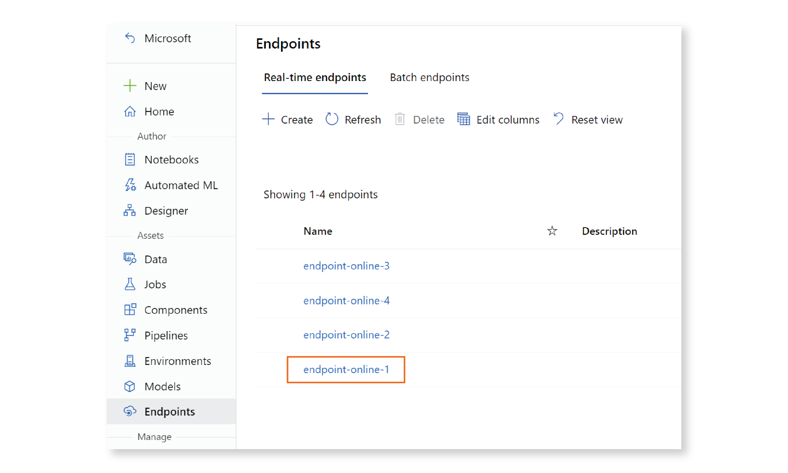
When running these commands, if you get an error saying that the endpoint name is already in use, you’ll need to edit the endpoint YAML file and choose a different name. Note that these resources take a little while to get created, especially the deployment. You can verify the endpoint’s creation by going to the Azure ML Studio, clicking on “Endpoints,” and making sure that you see the name of your endpoint listed on that page.
You can verify the deployment’s creation by clicking on the endpoint’s name and verifying that deployment “blue” is listed under “Deployment summary.”

Once your endpoint and deployment are created, you can invoke the endpoint:
az ml online-endpoint invoke --name endpoint-online-1 --request-file ../test_data/images_azureml.json
You should get a prediction similar to what you got on your development machine.
You may have noticed that we’re specifying a different input JSON file here, compared to our local prediction using the MLflow CLI. That’s because Azure ML requires this request file to consist of a dictionary with key “input_data.” Therefore, the images_azureml.json file contains a dictionary with key “input_data” and value equivalent to the contents of images.json. You can see below how these two files were generated in the generate_images.py file:
...
def get_dataframe_from_images() -> pandas.DataFrame:
    """
    Returns a pandas.DataFrame object that contains the images.
    """
    image_paths = [f for f in Path(IMAGES_DIR).iterdir() if Path.is_file(f)]
    image_paths.sort()

    df = pandas.DataFrame()
    for (i, image_path) in enumerate(image_paths):
        with Image.open(image_path) as image:
            x = np.asarray(image).reshape((1, -1)) / 255.0

            column_names = [f"col_{i}" for i in range(x.shape[1])]
            indices = [i]
            new_row_df = pandas.DataFrame(data=x,
                                          index=indices,
                                          columns=column_names)
            df = pandas.concat(objs=[df, new_row_df])

    return df


def generate_json_from_images() -> None:
    """
    Generates a json file from the images.
    """
    df = get_dataframe_from_images()

    data_json = df.to_json(orient="split")
    with open(Path(TEST_DATA_DIR, "images.json"), "wt",
              encoding="utf-8") as file:
        file.write(data_json)


def generate_json_for_azureml_from_images() -> None:
    """
    Generates a json file from the images, to be used when invoking the Azure ML
    endpoint.
    """
    df = get_dataframe_from_images()

    # pylint: disable=inconsistent-quotes
    data_json = '{"input_data":' + df.to_json(orient="split") + '}'
    with open(Path(TEST_DATA_DIR, "images_azureml.json"),
              "wt",
              encoding="utf-8") as file:
        file.write(data_json)
...
You can also invoke the endpoint using a POST command, in the command line or from within your code. In this case, you’ll need to specify a scoring URI (or REST endpoint) and a primary key. You can obtain this information using CLI commands, as you can see in the following invoke.sh script:
ENDPOINT_NAME=endpoint-online-1

SCORING_URI=$(az ml online-endpoint show --name $ENDPOINT_NAME --query scoring_uri -o tsv)
echo "SCORING_URI: $SCORING_URI"

PRIMARY_KEY=$(az ml online-endpoint get-credentials --name $ENDPOINT_NAME --query primaryKey -o tsv)
echo "PRIMARY_KEY: $PRIMARY_KEY"

OUTPUT=$(curl --location \
     --request POST $SCORING_URI \
     --header "Authorization: Bearer $PRIMARY_KEY" \
     --header "Content-Type: application/json" \
     --data @../test_data/images_azureml.json)
echo "OUTPUT: $OUTPUT"
Or you can obtain it from the Studio, in the endpoint’s “Consume” tab:

Once you’re done with endpoint 1, make sure you delete it to avoid getting charged:
az ml online-endpoint delete --name endpoint-online-1 -y
Endpoint 2 - Custom inference code
What if you wanted to add custom code during inference? That’s what endpoint 2 is about. We saw earlier that our model returns two dictionaries with keys corresponding to clothing items in the Fashion MNIST dataset, and values reflecting the likelihood of each clothing item being the correct prediction.
[
    {"0": -2.581446647644043, "1": -6.274104595184326, "2": -3.5508944988250732, "3": -4.623991012573242, "4": -4.489408493041992, "5": 5.361519813537598, "6": -3.7998995780944824, "7": 6.046654224395752, "8": 2.3112740516662598, "9": 7.203756332397461},
    {"0": 1.243371844291687, "1": -3.797163248062134, "2": 11.245864868164062, "3": 0.5872920155525208, "4": 5.921947002410889, "5": -11.618247032165527, "6": 5.215865612030029, "7": -6.385315418243408, "8": -1.7657241821289062, "9": -4.984302520751953}
]
In the output above, the first output dictionary has the highest value for item “9,” which corresponds to “Ankle boot,” and the second output dictionary has the highest value for item “2,” which corresponds to “Pullover.” If you’re planning to localize your client app, the current format might work just fine for you — you can simply convert each output dictionary to a localized string in the client app. But if you’ll be supporting a single language, you might want to convert each dictionary to the corresponding string on the server side, making it easier to consume on the client side.
Fortunately, MLflow allows us to create a model containing custom inference code. We can do this by saving the model using a “Python Function” flavor that contains the model we explored in endpoint 1 as an artifact, in addition to the custom inference code. Here’s the train.py file section that shows that:
...
def save_model(pytorch_model_dir: str, pyfunc_model_dir: str,
               model: nn.Module) -> None:
    """
    Saves the trained model.
    """
    # Save PyTorch model.
    pytorch_input_schema = Schema([
        TensorSpec(np.dtype(np.float32), (-1, 784)),
    ])
    pytorch_output_schema = Schema([TensorSpec(np.dtype(np.float32), (-1, 10))])
    pytorch_signature = ModelSignature(inputs=pytorch_input_schema,
                                       outputs=pytorch_output_schema)

    pytorch_code_filenames = ["neural_network.py", "utils_train_nn.py"]
    pytorch_full_code_paths = [
        Path(Path(__file__).parent, code_path)
        for code_path in pytorch_code_filenames
    ]
    logging.info("Saving PyTorch model to %s", pytorch_model_dir)
    shutil.rmtree(pytorch_model_dir, ignore_errors=True)
    mlflow.pytorch.save_model(pytorch_model=model,
                              path=pytorch_model_dir,
                              code_paths=pytorch_full_code_paths,
                              signature=pytorch_signature)

    # Save PyFunc model that wraps the PyTorch model.
    pyfunc_input_schema = Schema(
        [ColSpec(type="double", name=f"col_{i}") for i in range(784)])
    pyfunc_output_schema = Schema([TensorSpec(np.dtype(np.int32), (-1, 1))])
    pyfunc_signature = ModelSignature(inputs=pyfunc_input_schema,
                                      outputs=pyfunc_output_schema)

    pyfunc_code_filenames = ["model_wrapper.py", "common.py"]
    pyfunc_full_code_paths = [
        Path(Path(__file__).parent, code_path)
        for code_path in pyfunc_code_filenames
    ]
    model = ModelWrapper()
    artifacts = {
        ARTIFACT_NAME: pytorch_model_dir,
    }
    logging.info("Saving PyFunc model to %s", pyfunc_model_dir)
    shutil.rmtree(pyfunc_model_dir, ignore_errors=True)
    mlflow.pyfunc.save_model(path=pyfunc_model_dir,
                             python_model=model,
                             artifacts=artifacts,
                             code_path=pyfunc_full_code_paths,
                             signature=pyfunc_signature)
...
Notice that this time we call the function mlflow.pyfunc.save_model(), which saves the custom model using just the “Python Function” flavor. Our custom inference code is in model_wrapper.py (which we’ll see later in more detail) and common.py. Our non-custom model is added as an artifact to the custom model.
Notice also that custom PyTorch model and wrapper PyFunc model have different MLflow signatures. The PyFunc model will be invoked using a JSON file as input. In this case we use a ColSpec, list the column names in the JSON file, and specify that we expect type double because this is the type we get by default from JSON files. The PyTorch model will be invoked using a tensor, as you’ll see later in the model wrapper code. In this case we use a TensorSpec, and specify that it expects a tensor of shape (-1, 784) containing values with dtype float32.
This code generates the following directory structure:
pyfunc_model
    artifacts
        <a copy of the contents within the pytorch_model directory>
    code
        common.py
        model_wrapper.py
    conda.yaml
    MLmodel
    python_env.yaml
    requirements.txt
pytorch_model
    code
        neural_network.py
        utils_train_nn.py
    data
        model.pth
    conda.yaml
    MLmodel
    python_env.yaml
    requirements.txt
The pytorch_model directory contains the same model as endpoint 1. The pyfunc_model directory contains our custom model: it adds two extra files under “code” with our custom code, and contains the PyTorch model under “artifacts.” Let’s take a look at the model_wrapper.py file where you can find the code that wraps the PyTorch model as an artifact:
import logging

import mlflow
import pandas as pd
import torch

from common import ARTIFACT_NAME

labels_map = {
    0: 'T-Shirt',
    1: 'Trouser',
    2: 'Pullover',
    3: 'Dress',
    4: 'Coat',
    5: 'Sandal',
    6: 'Shirt',
    7: 'Sneaker',
    8: 'Bag',
    9: 'Ankle Boot',
}

class ModelWrapper(mlflow.pyfunc.PythonModel):
    """
    Wrapper for mlflow model.
    """

    def load_context(self, context: mlflow.pyfunc.PythonModelContext) -> None:
        self.model = mlflow.pytorch.load_model(context.artifacts[ARTIFACT_NAME])

    def predict(self, context: mlflow.pyfunc.PythonModelContext,
                model_input: pd.DataFrame) -> list[str]:
        with torch.no_grad():
            device = 'cuda' if torch.cuda.is_available() else 'cpu'
            logging.info('Device: %s', device)

            tensor_input = torch.Tensor(model_input.values).to(device)
            y_prime = self.model(tensor_input)
            probabilities = torch.nn.functional.softmax(y_prime, dim=1)
            predicted_indices = probabilities.argmax(1)
            predicted_names = [
                labels_map[predicted_index.item()]
                for predicted_index in predicted_indices
            ]
        return predicted_names
Subclassing mlflow.pyfunc.PythonModel enables us to create a custom MLflow model with the “Python Function” flavor — you can read more about it in the documentation. The load_context function is used to load any artifacts needed in predict — in our scenario we need to load the non-custom model. The predict function is called when MLflow makes a prediction, and that’s where we get to add any custom code we’d like. In this case, I make a prediction using the model obtained in load_context, then for each of the resulting dictionaries, I get the key associated with the maximum value, and use it to index into the labels_map dictionary in this file.
You can test this code on your development machine, using one of the following commands:
mlflow models predict --model-uri pyfunc_model --input-path "../test_data/images.csv" --content-type csv
mlflow models predict --model-uri pyfunc_model --input-path "../test_data/images.json" --content-type json
This time you should get strings representing clothing items as the output of your model prediction:
["Ankle Boot", "Pullover"]
To deploy this code in the cloud, you would follow exactly the same steps as endpoint 1.
Endpoint 3 - Token authentication
Endpoint 1 uses “key” authentication. With this authentication mode, when we invoke this endpoint using a POST command, we need to specify a scoring URI and a primary key that never expires. We can obtain this information using the CLI or by checking the Studio.
Endpoint 3 is similar to endpoint 1 except it uses “aml_token” authentication. With this authentication mode, when we invoke the endpoint using a POST command, we need to specify a scoring URI and an access token that expires after one hour. We can get this information using the CLI, as you can see in the following invoke.sh script:
ENDPOINT_NAME=endpoint-online-3

SCORING_URI=$(az ml online-endpoint show --name $ENDPOINT_NAME --query scoring_uri -o tsv)
echo "SCORING_URI: $SCORING_URI"

ACCESS_TOKEN=$(az ml online-endpoint get-credentials --name $ENDPOINT_NAME --query accessToken -o tsv)
echo "ACCESS_TOKEN: $ACCESS_TOKEN"

OUTPUT=$(curl --location \
     --request POST $SCORING_URI \
     --header "Authorization: Bearer $ACCESS_TOKEN" \
     --header "Content-Type: application/json" \
     --data @../test_data/images_azureml.json)
echo "OUTPUT: $OUTPUT"
Or we can get the scoring URI and an access token in the Studio, by going to “Endpoints,” clicking on the name of the endpoint and then on the “Consume” tab:

All other aspects of the creation and inference of this endpoint are the same as endpoint 1, so I won’t repeat them here.
Endpoint 4 - Multiple deployments
Endpoint 4 demonstrates how to ensure the safe rollout of a new deployment.
Let’s imagine a scenario where we used a managed online endpoint to deploy our PyTorch model using a machine with a CPU, but our team now decides that we need to use a GPU instead. We change the deployment to use a GPU, and that works fine in our internal testing. But the CPU-based endpoint is already in use by clients, and we don’t want to disrupt the service. Switching all clients to a new deployment is a risky move that may reveal issues and cause instability.
That’s where Azure ML’s safe rollout feature comes in. Instead of making an abrupt switch, we can use a “blue-green” deployment approach, where we roll out the new version of the code to a small subset of clients, and tune the size of that subset as we go. After ensuring that the clients calling the new version of the code encounter no issues for a while, we can increase the percentage of clients, until we’ve completed the switch.
Endpoint 4 in the accompanying project will demonstrate this scenario by specifying one endpoint with two deployments. Here are the contents of the endpoint.yml file:
$schema: https://azuremlschemas.azureedge.net/latest/managedOnlineEndpoint.schema.json
name: endpoint-online-4
auth_mode: key
Here are the contents of the deployment-blue.yml file:
$schema: https://azuremlschemas.azureedge.net/latest/managedOnlineDeployment.schema.json
name: blue
endpoint_name: endpoint-online-4
model: azureml:model-online-4@latest
instance_type: Standard_DS4_v2
instance_count: 1
And here are the contents of the deployment-green.yml file:
$schema: https://azuremlschemas.azureedge.net/latest/managedOnlineDeployment.schema.json
name: green
endpoint_name: endpoint-online-4
model: azureml:model-online-4@latest
instance_type: Standard_NC6s_v3
instance_count: 1
You can create the endpoint and deployments using the following CLI commands:
az ml online-endpoint create -f cloud/endpoint.yml
az ml online-deployment create -f cloud/deployment-blue.yml --all-traffic
az ml online-deployment create -f cloud/deployment-green.yml
We’ve specified that the “blue” deployment should receive 100% of the traffic, and the “green” deployment receives none. When you’re ready to adjust the traffic allocation, you can use the following command:
az ml online-endpoint update --name endpoint-online-4 --traffic "blue=90 green=10"
You can then keep adjusting the traffic until you’re ready to make the final switch.
For more information about safe rollout, check out the documentation.
Everything else about this endpoint is similar to endpoint 1, so I won’t repeat it here.
Conclusion
In this article, you learned how to deploy your MLflow model using managed online endpoints. You saw four different scenarios: a basic endpoint with “key” authentication, an endpoint with custom inference code, an endpoint with “aml_token” authentication, and a blue-green endpoint with safe rollout. You also saw some of the advantages of saving your model with MLflow: you can create a basic deployment without writing any inference code, and you don’t need to specify an environment in your deployment YAML. Hopefully you found this post informative.
Read next: Creating managed online endpoints in Azure ML without using MLflow