How to train using pipelines and components in Azure ML
Created:
Updated:
Topic: Azure ML: from beginner to pro
Introduction
Azure ML components and pipelines are useful if you have multiple steps in your training code that can be logically separated, especially if some of those steps can potentially be reused in the future. In this post, I’ll discuss how to break up your training code into components, and how to connect those components into a pipeline. If you’re already familiar with basic training and want to take your skills to the next level, then you’re in the right place. If you’re hoping to learn how to do basic training in Azure ML, I recommend that you read my post on the topic.
I created two GitHub repos to illustrate the ideas in this post. The first GitHub repo shows how to work with pipelines and components using the CLI, and the second GitHub repo shows the same steps using the Python SDK. If you need a refresher on the different methods for creating resources in Azure ML, I recommend reading my introduction to Azure ML article.
For Azure and project setup, please refer to the README files of each GitHub repo. You’ll also find there a reference list of all the commands explained in this post.
Training and inference on your development machine
Components and pipelines are useful to break up the execution of your machine learning code into steps. One common scenario is to break up our work into two steps: a training step where we train and validate our model, and a test step where we test your model using data that was not seen during training. This is the scenario I’ll be demonstrating in this blog post. But components and pipelines are a great tool for any other scenario where your code can be broken into steps. For example, you may have one or more blocks of data pre-processing code.
You can see how I developed code for the train and test steps in the CLI GitHub repo associated with this post:
- The training step splits the training data into validation and training sets, wraps them with DataLoaders that load one minibatch of data at a time, uses the backpropagation algorithm to train the model using all batches for several epochs, reports on the training and validation accuracy and loss, and saves the trained model using MLflow.
- The test step wraps the test data with a DataLoader, loads the trained model, runs the model using the test data, and reports on the accuracy and loss of the model’s prediction. Since we saved our model using MLflow, we could have used the mlflow.evalute function from the MLflow API to evaluate the model, instead of our custom code. But because this function is still experimental at the time of writing, I decided to show you custom code instead. In the future, I think that using the MLflow API is the way to go because of the great logging support it provides.
In VS Code, select the run configuration “Train locally” and press F5 to train on your development machine. Then repeat for “Test locally.” You can look at the logs generated by the code in these files with the following command:
mlflow ui
The test step should give you a test accuracy of 84 or 85%.
Creating components
Once we’ve written and tested the code for the training and test steps, we’re ready to run it in the cloud. Since our training code was organized into two steps with distinct logic, we would like to maintain that separation in the cloud. That’s where components come in.
An Azure ML component is a reusable piece of code with inputs and outputs — it’s basically like a function in any programming language. In Azure ML, each component needs to be defined in its own Python file. Inputs and outputs are specified as command line arguments. For example, notice that train.py has two command line arguments: the path to the directory where our training data is located, and the path to the directory where it will save the trained model.
def main() -> None:
    (...)

    parser = argparse.ArgumentParser()
    parser.add_argument("--data_dir", dest="data_dir", default=DATA_DIR)
    parser.add_argument("--model_dir", dest="model_dir", default=MODEL_DIR)
    args = parser.parse_args()
    logging.info("input parameters: %s", vars(args))

    (...)
The data_dir argument is an input to this component, because that’s where the input data is located. On the other hand, model_dir is an output of the component, because it represents the path where we want to save the model trained by the code (which is the output of this component).
We can represent this information in train.yml, the YAML file containing the train component specification:
$schema: https://azuremlschemas.azureedge.net/latest/commandComponent.schema.json
name: component_pipeline_cli_train
version: 1
type: command

inputs:
  data_dir:
    type: uri_folder

outputs:
  model_dir:
    type: mlflow_model

environment:
  image: mcr.microsoft.com/azureml/openmpi4.1.0-ubuntu20.04:latest
  conda_file: conda.yml

code: ../src
command: >-
  python train.py --data_dir ${{inputs.data_dir}} --model_dir ${{outputs.model_dir}}
As you can see, the names of the input and the output in the component YAML speficication match the names of the arguments in the code. The only difference is that in the YAML we’re explicit about which arguments are inputs to the component and which ones are outputs. Notice that along with the input and output names, I specify their types. To see the list of all supported types, delete the current type and press Ctrl + Space in VS Code. Here’s the list of supported input types:

And here’s the list of supported output types:

The YAML for the component also specifies the sofware environment we need to have installed on the virtual machine where the code will run — you can read more about this in my blog post about environments. It also contains the local folder where the code for the component is located, and the command used to run it. The command in this file says that I want to run the train.py file by passing the data_dir input and model_dir output as arguments. Notice the $${{...}} special syntax used to refer to inputs and outputs:
python train.py --data_dir ${{inputs.data_dir}} --model_dir ${{outputs.model_dir}}
You can learn more about the Command Component YAML schema in the docs.
You’re now ready to create the component in Azure ML, which you can do by executing the following command in the terminal:
az ml component create -f cloud/train.yml
You can verify that your component was created by going to the Azure ML Studio, clicking on “Components”, and looking for a component with name “component_pipeline_cli_train”, which is the name we specified in the YAML file.
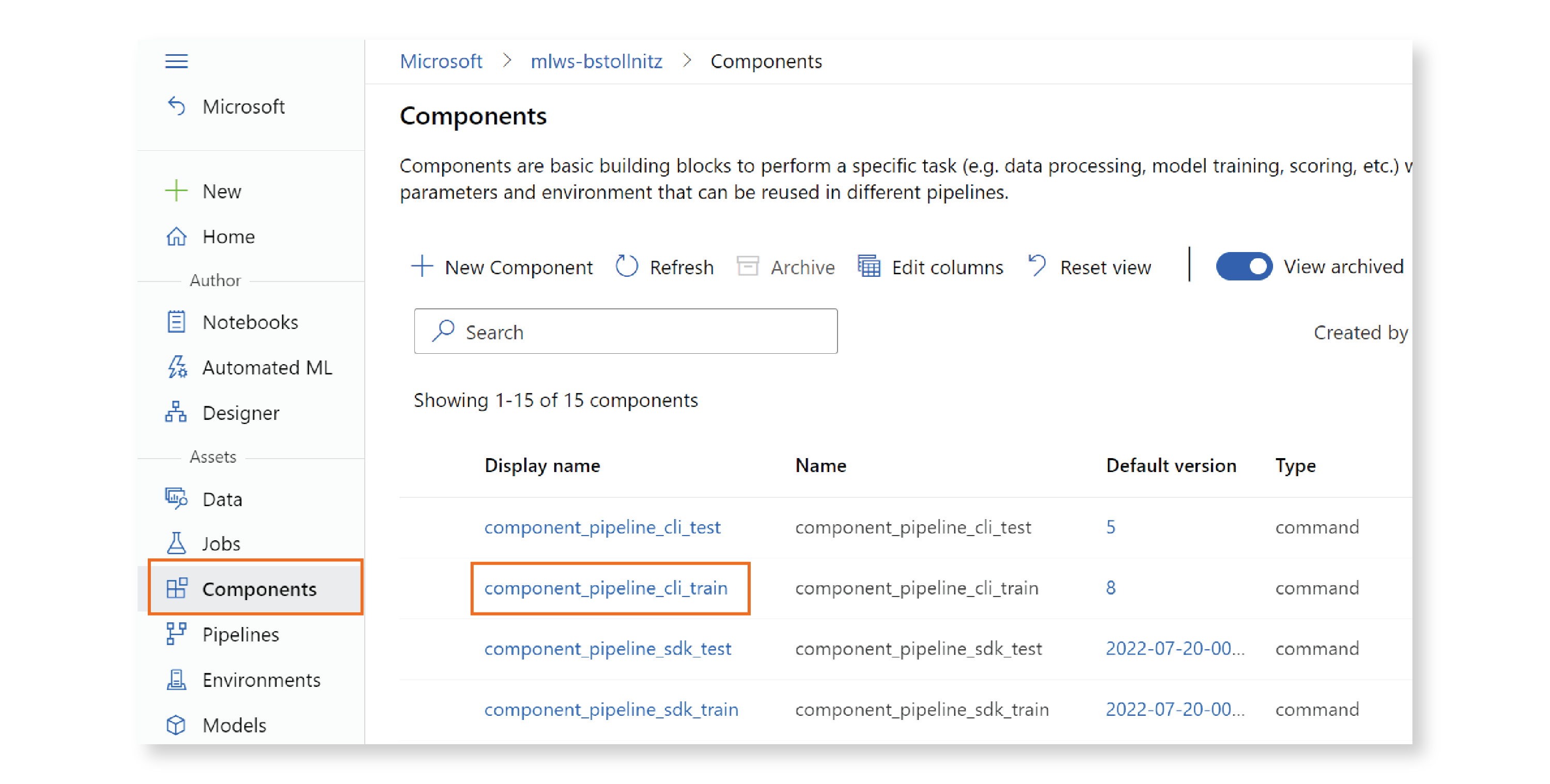
The train component is created in the cloud! Since our code is nicely encapsulated by a well-defined interface, we can easily reuse it in other projects. This is one of the many advantages of using components!
The test component is very similar. The code file test.py has two arguments: the path to the trained model, and the path to the test data.
def main() -> None:
    (...)

    parser = argparse.ArgumentParser()
    parser.add_argument("--data_dir", dest="data_dir", default=DATA_DIR)
    parser.add_argument("--model_dir", dest="model_dir", default=MODEL_DIR)
    args = parser.parse_args()
    logging.info("input parameters: %s", vars(args))

    (...)
In this case, both arguments are inputs because the trained model and the test data already exist, and are not generated by the component. This is reflected in the test.yml YAML file:
$schema: https://azuremlschemas.azureedge.net/latest/commandComponent.schema.json
name: component_pipeline_cli_test
version: 1
type: command

inputs:
  data_dir:
    type: uri_folder
  model_dir:
    type: mlflow_model

environment:
  image: mcr.microsoft.com/azureml/openmpi4.1.0-ubuntu20.04:latest
  conda_file: conda.yml

code: ../src
command: >-
  python test.py --model_dir ${{inputs.model_dir}} --data_dir ${{inputs.data_dir}}
This time the YAML specification contains two inputs, and no outputs. We’ll log the test accuracy and loss, so we don’t need to return them as output. Just like before, we execute the following command to create the component in the cloud:
az ml component create -f cloud/test.yml
And we verify that our component was created in the studio:
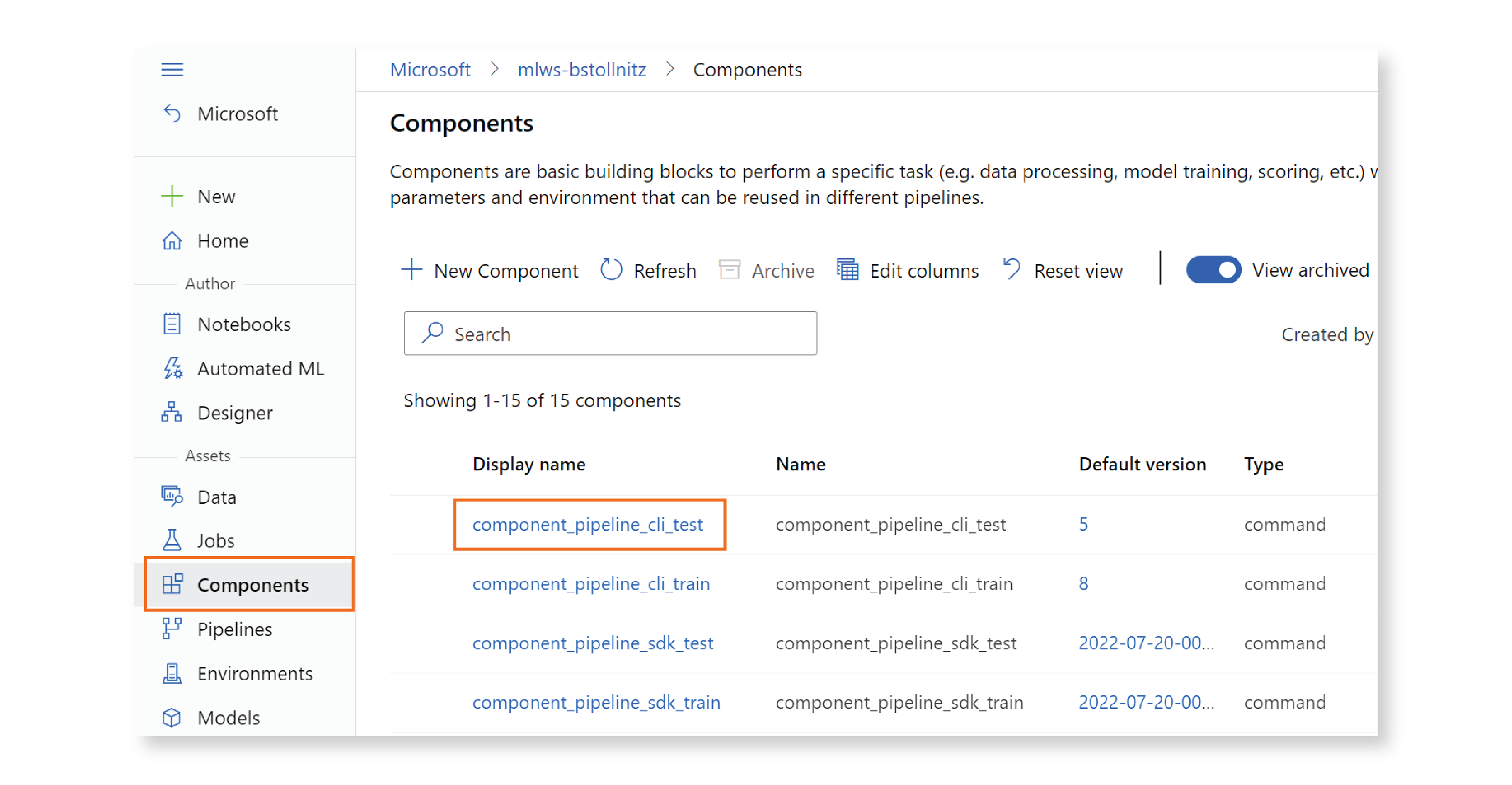
Great! Our two components are now registered in Azure ML.
Creating a pipeline
How do we run our components? We first need to create a pipeline that defines our workflow by specifying dependencies between our components. Then we can run the pipeline directly — a pipeline is just a type of job, so we can run it like any other job! (If you need to remind yourself of the Azure ML resource hierarchy, you can take a look at my Azure ML overview blog post.)
Before we can create our pipeline, we need to create two other resources that it will depend on: a compute cluster that specifies the hardware we want to run on, and a dataset with our training and test data. Let’s start by creating a compute cluster of up to 4 CPU VMs. Here’s the YAML definition for this cluster, which can be found in the cluster-cpu.yml file:
$schema: https://azuremlschemas.azureedge.net/latest/amlCompute.schema.json
name: cluster-cpu
type: amlcompute
size: Standard_DS4_v2
min_instances: 0
max_instances: 4
And here’s the CLI command to create this resource in the cloud:
az ml compute create -f cloud/cluster-cpu.yml
If you want to learn more about the different types of compute supported on Azure ML, you can consult my blog post on the topic.
Next we’ll create the dataset. The YAML definition can be found in data.yml:
$schema: https://azuremlschemas.azureedge.net/latest/data.schema.json
name: data-fashion-mnist
description: Fashion MNIST Dataset.
path: ../data/
And here’s the CLI command.
az ml data create -f cloud/data.yml
We have everything we need to create our pipeline. In our scenario, we have a very simple pipeline that takes the data as input, executes our train and test components, and produces a trained model as output. Here’s a diagram representing our pipeline:

The dataset is used as input to both models because it contains both the training and test data. The train component is executed first, and it ouputs a trained model, which is used both as input to the test component and as output to the whole pipeline. The test component takes as input the data and the trained model, and produces no outputs, just useful logs. This is a very simple pipeline, but you can imagine how these can get arbitrarily complex, depending on how many components you have and the interdependencies between them.
Let’s take a look at pipeline-job.yml, the YAML file that specifies the details for the pipeline creation:
$schema: https://azuremlschemas.azureedge.net/latest/pipelineJob.schema.json
type: pipeline
experiment_name: aml_pipeline_cli

compute: azureml:cluster-cpu

inputs:
  data_dir:
    path: azureml:data-fashion-mnist@latest
    type: uri_folder

outputs:
  model_dir:
    type: mlflow_model

jobs:
  train:
    type: command
    component: azureml:component_pipeline_cli_train@latest
    inputs:
      data_dir: ${{parent.inputs.data_dir}}
    outputs:
      model_dir: ${{parent.outputs.model_dir}}

  test:
    type: command
    component: azureml:component_pipeline_cli_test@latest
    inputs:
      data_dir: ${{parent.inputs.data_dir}}
      model_dir: ${{parent.jobs.train.outputs.model_dir}}
Once again, we use the $${...} syntax to refer to the inputs and ouputs of the pipeline. We also use the same syntax within the test component, to specify that the model_dir input should be the output of the train component:
model_dir: ${{parent.jobs.train.outputs.model_dir}}
These input and output dependencies define the shape of our pipeline, and help Azure ML determine whether different components can run in parallel or need to run sequentially.
We’re now ready to run our pipeline in the cloud:
run_id=$(az ml job create -f cloud/pipeline-job.yml --query name -o tsv)
The --query parameter specifies that we want to query the JSON returned by the command using JMESPath language, as you can see in the documentation for the “az ml job create” command. We specify that we want to extract the value associated with the “name” key from the returned JSON. The -o parameter specifies that we want the output to be formatted using tab-separated values — you can learn more about output formats in the documentation. The result of applying these two parameters to our command is the ID for this particular job instance — we’ll need this later. If we execute the same command again, we would get a different instance of the same job definition, with a different run ID.
This job will take a while to execute. You can go to the studio, click on “Jobs,” then “aml_pipeline_cli,” which is the name we specified for the experiment in the job YAML file. An experiment is just a collection of jobs. Once the status of the latest job displays “Completed,” you’re ready to proceed.
We can then register the trained model returned by the pipeline with Azure ML. We’ll use the following command to do that:
az ml model create --name model-pipeline-cli --version 1 --path "azureml://jobs/$run_id/outputs/model_dir" --type mlflow_model
I could have used a separate YAML file to aid in the creation of the model, but since we need just a few properties, defining it inline works too. You can go to the studio and click on “Models” to make sure that your model is created correctly.
Next we’ll deploy the registered model using a managed online endpoint and deployment. The file endpoint.yml contains the YAML definition for the endpoint:
$schema: https://azuremlschemas.azureedge.net/latest/managedOnlineEndpoint.schema.json
name: endpoint-pipeline-cli
auth_mode: key
And deployment.yml contains the YAML definition for the deployment:
$schema: https://azuremlschemas.azureedge.net/latest/managedOnlineDeployment.schema.json
name: blue
endpoint_name: endpoint-pipeline-cli
model: azureml:model-pipeline-cli@latest
instance_type: Standard_DS4_v2
instance_count: 1
And here’s how we can create them in the cloud:
az ml online-endpoint create -f cloud/endpoint.yml
az ml online-deployment create -f cloud/deployment.yml --all-traffic
Last, we can invoke the endpoint:
az ml online-endpoint invoke --name endpoint-pipeline-cli --request-file test_data/images_azureml.json
Although this is not necessary for deployment, we can use the run ID we got earlier to download the trained model:
az ml job download --name $run_id --output-name "model_dir"
Once you’re done with the endpoint, make sure you delete it to avoid getting charged unnecessarily:
az ml online-endpoint delete --name endpoint-pipeline-cli -y
And you’re done! This post explains how to train a model with components and a pipeline using the CLI, but you can perform the exact same steps in code using the Azure ML Python SDK. I won’t go into detail, but my second GitHub repo associated with this post shows how to use the Python SDK. If you understand how to accomplish this scenario using the CLI, the SDK version should be self-explanatory. You could also perform all the same steps using the studio UI.
Conclusion
In this post, you learned how to organize your training code into reusable components with inputs and outputs, and how to connect those components using a pipeline. You then ran the pipeline in the cloud, and deployed the trained model generated by the pipeline. I hope that this information has improved your productivity with Azure ML.