Bea Stollnitz - Introduction to PyTorch

Introduction

Today Microsoft and PyTorch announced a “PyTorch Fundamentals” tutorial, which you can find on Microsoft’s site and on PyTorch’s site. The code in this post is based on the code appearing in that tutorial, and forms the foundation for a series of other posts, where I’ll explore other machine learning frameworks and show integration with Azure ML.

In this post, I’ll explain how you can create a basic neural network in PyTorch, using the Fashion MNIST dataset as a data source. The neural network we’ll build takes as input images of clothing, and classifies them according to their contents, such as “Shirt,” “Coat,” or “Dress.”

I’ll assume that you have a basic conceptual understanding of neural networks, and that you’re comfortable with Python, but I assume no knowledge of PyTorch.

The code for this post can be found on GitHub.

Data

Let’s first get the imports for the code in the main.py file, which contains most of the code in this blog post.

https://github.com/bstollnitz/fashion-mnist-pytorch/tree/main/fashion-mnist-pytorch/src/main.py

from typing import Tuple

import numpy as np
import torch
from PIL import Image
from torch import nn
from torch.nn.modules.loss import CrossEntropyLoss
from torch.optim import Optimizer
from torch.utils.data import DataLoader
from torchvision import datasets
from torchvision.transforms import ToTensor

from neural_network import NeuralNetwork
...

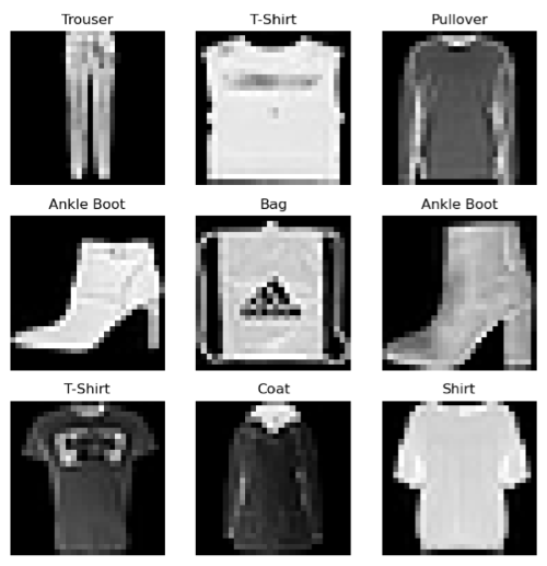
Now we’ll get familiar with the data we’ll be using, the Fashion MNIST dataset. This dataset contains 70,000 grayscale images of articles of clothing — 60,000 meant to be used for training and 10,000 meant for testing. The images are square and contain 28 × 28 = 784 pixels, where each pixel is represented by a value between 0 and 255. Each of these images is associated with a label, which is an integer between 0 and 9 that classifies the article of clothing. The following dictionary helps us understand the clothing categories corresponding to these integer labels:

https://github.com/bstollnitz/fashion-mnist-pytorch/tree/main/fashion-mnist-pytorch/src/main.py

...
labels_map = {
    0: 'T-Shirt',
    1: 'Trouser',
    2: 'Pullover',
    3: 'Dress',
    4: 'Coat',
    5: 'Sandal',
    6: 'Shirt',
    7: 'Sneaker',
    8: 'Bag',
    9: 'Ankle Boot',
}
...

Here’s a random sampling of 9 images from the dataset, along with their labels:

Sample of the Fashion MNIST dataset.

PyTorch Tensor

A PyTorch tensor is the data structure used to store the inputs and outputs of a deep learning model, as well as any parameters that need to be learned during training. It’s a super important concept to understand if you’re going to be working with PyTorch.

Mathematically speaking, a tensor is just a generalization of vectors and matrices. A vector is a one-dimensional array of values, a matrix is a two-dimensional array of values, and a tensor is an array of values with any number of dimensions. A PyTorch tensor, much like NumPy’s ndarray, gives us a way to represent multidimensional data, but with added tricks, such as the ability to perform operations on a GPU and the ability to calculate derivatives.

Suppose we want to represent this 3 × 2 matrix in PyTorch:

Here’s the code to create the corresponding tensor:

X = torch.tensor([[1, 2], [3, 4], [5, 6]])

We can inspect the tensor’s shape attribute to see how many dimensions it has and the size in each dimension. The device attribute tells us whether the tensor is stored on the CPU or GPU, and the dtype attribute indicates what kind of values it holds. We use the type() method to check the type of the tensor itself.

print(X.shape)
print(X.device)
print(X.dtype)
print(X.type())

torch.Size([3, 2])
cpu
torch.int64
torch.LongTensor

If you consult this table in the PyTorch docs, you’ll see that this all makes sense: a tensor with a dtype of torch.int64 on the CPU has a type of torch.LongTensor.

There are many ways to move this tensor to the GPU (assuming that you have a GPU and CUDA setup on your machine). One way is to change its device to 'cuda':

device = 'cuda' if torch.cuda.is_available() else 'cpu'
X = X.to(device)
print(X.device)
print(X.type())

cuda:0
torch.cuda.LongTensor

If you’ve used NumPy ndarrays before, you might be happy to know that PyTorch tensors can be indexed in a familiar way. We can slice a tensor to view a smaller portion of it:

X = X[0:2, 0:1]

We get this:

We can also convert tensors to and from NumPy arrays, and have a NumPy ndarray and PyTorch tensor share the same underlying memory (as long as the tensor is on the CPU, just like the ndarray):

X = X[0:2, 0:1].cpu()       # [1, 3] on the CPU
array = X.numpy()           # [1, 3]
Y = torch.from_numpy(array) # [1, 3]
array[0, 0] = 2             # [2, 3]
print(X)
print(Y)

tensor([[2],
        [3]])
tensor([[2],
        [3]])

If your tensor contains a single value, the item() method is a handy way to get that value as a scalar:

Z = torch.tensor([6])
scalar = Z.item()
print(scalar)

I mentioned earlier that tensors also help with calculating derivatives. I will explain how that works later in this post, in the section titled PyTorch autograd on a simple scenario.

PyTorch DataLoader, Dataset, and data transformations

Let’s start by defining a few constants that we’ll use throughout the project.

https://github.com/bstollnitz/fashion-mnist-pytorch/tree/main/fashion-mnist-pytorch/src/main.py

...
DATA_DIRPATH = 'fashion-mnist-pytorch/data'
MODEL_DIRPATH = 'fashion-mnist-pytorch/model'
IMAGE_FILEPATH = 'fashion-mnist-pytorch/src/predict-image.png'
...

PyTorch’s torchvision package gives us a super easy way to get the Fashion MNIST data, by simply instantiating the datasets.FashionMNIST class. Let’s take a look at the code.

https://github.com/bstollnitz/fashion-mnist-pytorch/tree/main/fashion-mnist-pytorch/src/main.py

def _get_data(batch_size: int) -> Tuple[DataLoader, DataLoader]:
    """Downloads Fashion MNIST data, and returns two DataLoader objects
    wrapping test and training data."""
    training_data = datasets.FashionMNIST(
        root=DATA_DIRPATH,
        train=True,
        download=True,
        transform=ToTensor(),
    )

    test_data = datasets.FashionMNIST(
        root=DATA_DIRPATH,
        train=False,
        download=True,
        transform=ToTensor(),
    )

    train_dataloader = DataLoader(training_data,
                                  batch_size=batch_size,
                                  shuffle=True)
    test_dataloader = DataLoader(test_data, batch_size=batch_size, shuffle=True)

    return (train_dataloader, test_dataloader)

The root parameter specifies the local path where we want the data to go; train should be set to True to get the training set, and to False to get the test set; download is set to True to ensure that the data is downloaded to the location specified in root; and transform contains any transformations we want to perform on the data.

In this case, we apply a ToTensor() transform, which does two things:

Converts each image into a PyTorch tensor, whose shape is [number of channels, height, width]. If we were working with color images, we’d have three channels (red, green, and blue). But because our images are black and white, the number of channels is one. Height and width are both 28 pixels in our scenario, so the shape of each of our images is [1, 28, 28].
Converts the value of each pixel from integers between 0 and 255 into floating-point numbers between 0 and 1.

The datasets.FashionMNIST class derives from Dataset, a base class provided by PyTorch for holding data. If we were using custom data, we would have to create our own class that derives from Dataset and override two functions: __len__(self) returns the length of the dataset, and __getitem__(self, idx) returns the item corresponding to an index. In our scenario, torchvision makes life easy for us by giving us the data already contained in a Dataset.

We then wrap the training and test datasets into instances of the DataLoader class, which gives us an iterable over the Dataset. If we were to write a for loop over one of these DataLoader instances, each iteration would retrieve the next batch of images and corresponding labels in the Dataset, where the number of images is determined by the batch_size parameter passed to the DataLoader constructor. This functionality will be important later, when we train our model — we’ll come back to it.

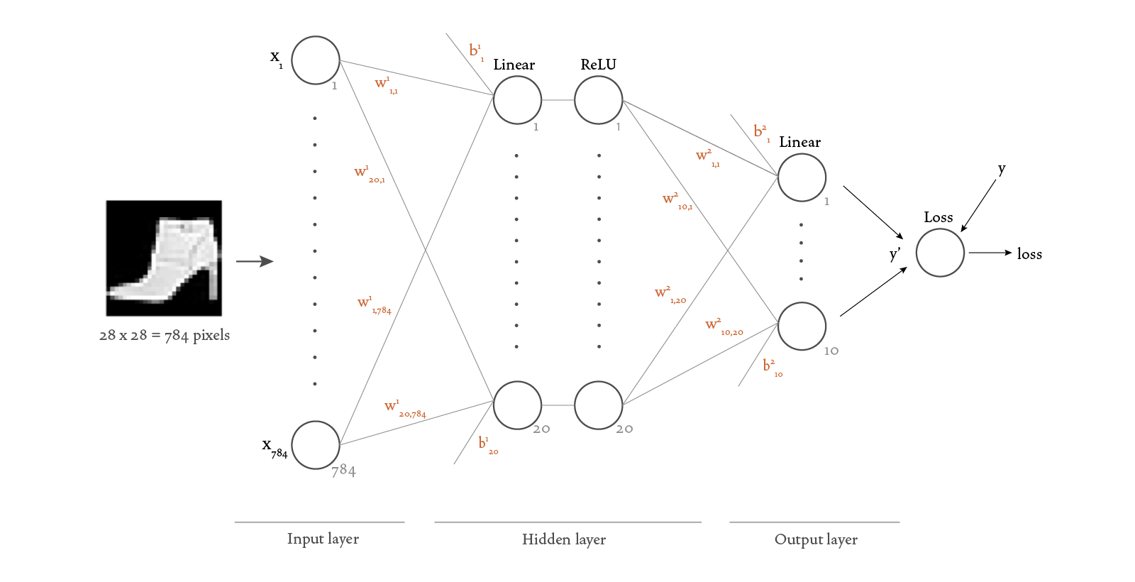
The neural network architecture

Our goal is to classify an input image into one of the 10 classes of clothing, so we will define our neural network to take as input a tensor of shape [1, 28, 28] and output a vector of size 10, where the index of the largest value in the output corresponds to the integer label for the class of clothing in the image. For example, if we use an image of an ankle boot as input, we might get an output vector like this:

In this particular example, the largest value appears at index 9 (counting from zero) — and as we showed in the Data section above, index 9 corresponds to the “Ankle Boot” category. So this indicates that our neural network correctly classified the image of an ankle boot.

Here’s a visualization of the structure of the neural network we chose for this scenario:

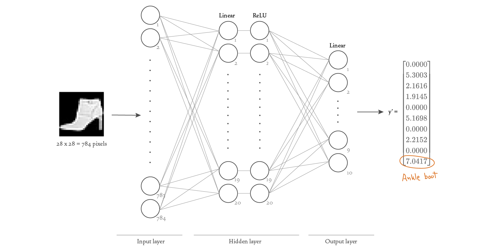
Diagram of Fashion MNIST classification neural network.

Because each image has 28 × 28 = 784 pixels, we need 784 nodes in the input layer (one for each pixel value). We decided to add one hidden layer with 20 nodes, with each node followed by a ReLU (rectified linear unit) activation function. We want the output of our network to be a vector of size 10, therefore our output layer needs to have 10 nodes.

In PyTorch, a neural network is defined as a class that derives from the nn.Module base class. Here’s the code that represents our network design:

https://github.com/bstollnitz/fashion-mnist-pytorch/tree/main/fashion-mnist-pytorch/src/neural_network.py

import torch
from torch import nn

class NeuralNetwork(nn.Module):
    """Neural network that classifies Fashion MNIST-style images."""

    def __init__(self):
        super().__init__()
        self.sequence = nn.Sequential(nn.Flatten(), nn.Linear(28 * 28, 20),
                                      nn.ReLU(), nn.Linear(20, 10))

    def forward(self, x: torch.Tensor) -> torch.Tensor:
        y_prime = self.sequence(x)
        return y_prime

The Flatten layer turns our input tensor of shape [1, 28, 28] into a vector of size 728. The Linear layers are also known as “fully connected” or “dense” layers because they connect all nodes from the previous layer with each of their own nodes — notice how each Linear constructor is passed the size of the previous layer and the size of the current layer. The ReLU layers take the output of the previous layer and pass it through a “Rectified Linear Unit” activation function, which adds non-linearity to the computation. The Sequential class combines all the other layers. Lastly, we define the forward method, which supplies a tensor x as input to the sequence of layers and produces the y_prime vector as a result.

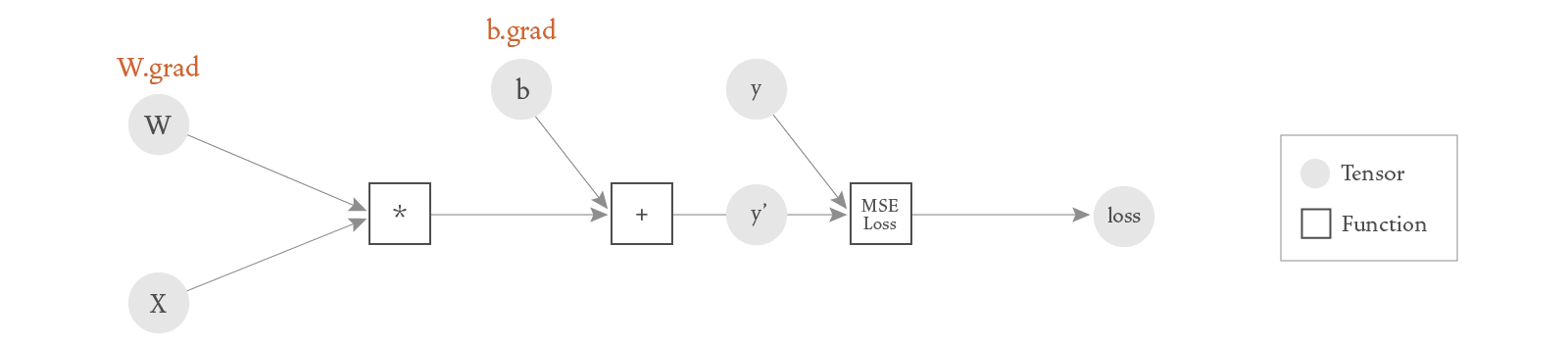
PyTorch autograd on a simple scenario

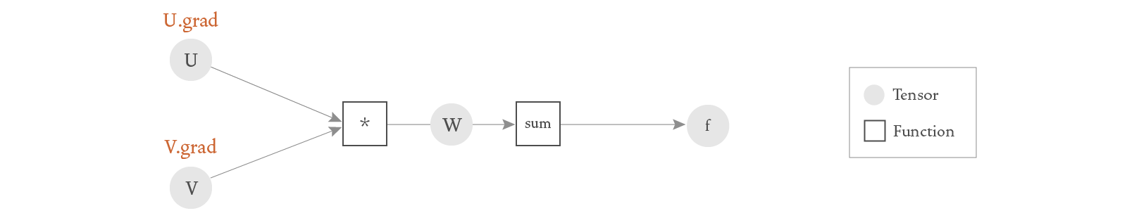
Now that we have a neural network model, we’re interested in training it — but part of the training process requires calculating derivatives that involve tensors. So let’s learn about PyTorch’s built-in automatic differentiation engine, autograd, using a very simple example. Let’s consider the following two tensors:

Now let’s suppose that we want to multiply by , and then sum all the values in the resulting tensor, such that the result is a scalar. In math notation, we might represent this as the following scalar function :

Our goal is to calculate the derivative of with respect to each of its inputs: and . We’ll start by setting the requires_grad flag to true during the construction of the tensors to tell autograd to help us calculate those derivatives. Then, when we execute a function that takes our tensors as input, autograd records any information necessary to compute the derivative of that function with respect to our tensors. Calling backward() on the output tensor then kicks off the actual computations of those derivatives. Afterwards, we can access the derivatives by inspecting the grad attribute of each input tensor.

# Decimal points in tensor values ensure they are floats, which autograd requires.
U = torch.tensor([[1., 2.]], requires_grad=True)
V = torch.tensor([[3., 4.], [5., 6.]], requires_grad=True)
W = torch.matmul(U, V)
f = W.sum()
f.backward()
print(U.grad)
print(V.grad)

tensor([[ 7., 11.]])
tensor([[1., 1.],
        [2., 2.]])

Internally, a dynamic directed acyclic graph (DAG) of instances of type Function is created to represent the operations we’re performing on our tensors. These Function instances have a forward method that, given one or more inputs, executes the computations needed to produce an output. And they have a backward method that calculates the derivatives of the function with respect to each of its inputs. The diagram below illustrates the DAG that corresponds to our current example. Instances of type Tensor flow left-to-right as the functions are being executed, and right-to-left as the derivatives are being calculated.

Tensor calculations represented as a DAG.

Let’s take a look at the math used to compute the derivatives. You only need to understand matrix multiplication and partial derivatives to follow along, but if the math isn’t as interesting to you, feel free to skip to the next section.

We’ll start by thinking of and as generic 1 × 2 and 2 × 2 matrices:

Then the scalar function can be written as:

We can now calculate the derivatives of with respect to each of its inputs:

As you can see, when we plug in the numerical values of and , we get the same result that PyTorch’s autograd gave for U.grad and V.grad.

PyTorch autograd on a neural network

We saw how automatic differentiation works for a simple calculation. Let’s now explore how it works for a neural network. We’ll consider a very small neural network, consisting of an input layer and an output layer, with no hidden layers:

Diagram of a basic neural network.

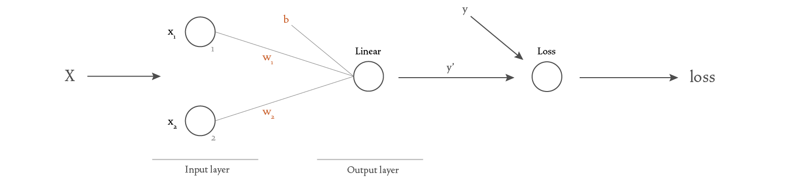
When training a neural network, our goal is to find parameter values that will enable the network to produce predicted labels as similar as possible to the actual labels provided in the training data. In our current very small network, the parameters include two weights and and a bias value associated with the linear layer. And training proceeds by minimizing a “loss” function, which measures the dissimilarity between predicted values and actual values . Let’s include the weights, bias, and loss function in a more detailed diagram:

Diagram of a basic neural network with more detail.

Let’s now analyze the calculations that happen when we give it some input data. We can represent the input data and weights as vectors:

The calculations in the linear layer give us the predicted value :

We’ll use the MSELoss function to calculate the loss as the mean squared error:

The DAG for this simple neural network should now be easy to understand:

DAG corresponding to a basic neural network.

In the scenarios shown here, our graphs are really just simple trees. But as you can imagine, when building larger neural networks, the complexity of these graphs increases.

Technically, you could write the code for this simple neural network by spelling out all the individual operations, as in the code sample below. However, you typically wouldn’t — you would instead create a neural network similar to the one I showed earlier, but with a single Linear layer. Creating a neural network with a Linear layer is a simpler solution with a higher level of abstraction, and therefore scales better to more complex networks. But for now, let’s write out all the steps:

W = torch.tensor([[1., 2.]], requires_grad=True)
X = torch.tensor([[3.], [4.]])
b = torch.tensor([5.], requires_grad=True)
y = torch.tensor([[6.]])
y_prime = torch.matmul(W, X) + b
loss_fn = torch.nn.MSELoss()
loss = loss_fn(y_prime, y)
loss.backward()
print(W.grad)
print(b.grad)

tensor([[60., 80.]])
tensor([20.])

Setting requires_grad to True for a particular tensor should only be done when we need to calculate the gradient with respect to that tensor, because it adds a bit of overhead to the forward pass. Notice that in the code above, I only add requires_grad to the and weights, not the input and expected output . That’s because when training a neural network, we only need to calculate and , and no other derivatives. I’ll come back to this in the next section.

Also, there are some scenarios where we want to do a forward pass in the neural network without calculating any of the gradients. For example, when we want to test the network, or make a prediction, or fine tune an already-trained network. In those scenarios, we can wrap the operations with a torch.no_grad(), which tells autograd to skip any gradient-related setup in the forward pass.

U = torch.tensor([[1., 2.]], requires_grad=True)
V = torch.tensor([[3., 4.], [5., 6.]], requires_grad=True)
W = torch.matmul(U, V)
print(W.requires_grad)

with torch.no_grad():
  W = torch.matmul(U, V)
print(W.requires_grad)

True
False

One interesting property of PyTorch DAGs is that they are dynamic. This means that after each forward and backward pass, we’re free to change the structure of the graph and the shape of the tensors that flow through it, because the graph will be re-created in the next pass. This is a very powerful feature that allows tremendous flexiblity when training a model.

Training the network

In order to understand what happens during training, we need to add a little bit more detail to our neural network visualization.

Basic neural network with details.

There’s a lot of new information in this diagram, so I’ll expand on the new concepts here.

Notice that we’ve added weights to the connections between layers, and bias as input to Dense layers — and are the neural network’s parameters. Our goal when training our network (also known as fitting) is to find the parameters and that minimize the differences between the actual and predicted labels for our data.

Notice also that we added a Loss function to the diagram. This function takes in the outputs of the model (the predicted labels) and the actual labels , measures their differences, and combines those into a single output, which we call the loss. The loss gives us a single number that quantifies how similar our predictions are to the actual labels: a high loss indicates that they’re different, and a low loss indicates that our predictions are accurate. There are many ways to write this function, and in this sample we’ll use the CrossEntropyLoss, which is provided to us by PyTorch.

Mathematically speaking, we can now think of our neural network as a function that takes as input the data , expected labels , and parameters and , then performs a sequence of operations on that data, and returns a loss.

Our goal is to find the parameters and that lead to the lowest possible loss. (We can’t change our data or the corresponding labels — they’re fixed — but we can adjust and .) It turns out that problems of this kind fall in the well-studied mathematical area of optimization. And better yet, the simplest possible optimization technique, gradient descent, is easy to understand and often good enough for our purposes.

To implement the gradient descent algorithm, we iteratively improve our estimates of and according to the update formulas below, until the gradients are smaller than a pre-defined threshold (or for a pre-defined number of times):

The parameter is typically referred to as the “learning rate,” and will be defined later in the code. How do we calculate the derivatives needed in the gradient descent? We use the differentiation capabilities provided by autograd, which we learned in the previous section.

When we put all of these ideas together, we get the backpropagation algorithm. This algorithm consists of four steps:

a forward pass through the model to compute the predicted value, y_prime = model(X)
a calculation of the loss using a loss function, loss = loss_fn(y_prime, y)
a backward pass from the loss function through the model to calculate derivatives, loss.backward()
a gradient descent step to update and using the derivatives calculated in the backward pass, optimizer.step()

Here’s the complete code:

https://github.com/bstollnitz/fashion-mnist-pytorch/tree/main/fashion-mnist-pytorch/src/main.py

...
def _fit_one_batch(x: torch.Tensor, y: torch.Tensor, model: NeuralNetwork,
                   loss_fn: CrossEntropyLoss,
                   optimizer: Optimizer) -> Tuple[torch.Tensor, torch.Tensor]:
    """Trains a single minibatch (backpropagation algorithm)."""
    y_prime = model(x)
    loss = loss_fn(y_prime, y)

    optimizer.zero_grad()
    loss.backward()
    optimizer.step()

    return (y_prime, loss)
...

The reason we call zero_grad() before the backward pass is a bit of a technicality. During the backward pass, gradients are accumulated by adding them to the grad attribute of a tensor, so we need to explicitly ensure that the grad attribute of each parameter is reset to zero before this pass.

You might be wondering how many images we pass as our input . A single image? All 60,000 images? Doing a complete backpropagation step (forward, backward, and optimizer step) for each individual image would be inefficient because we would have to perform all the calculations 60,000 times in order to account for every input image. If we included all the input images in , we’d need a lot of memory, and we’d spend a lot of time computing the forward pass just to take a single gradient descent step. So we settle for a size in between, called the “mini-batch” size. You might recall that when we created DataLoader instances, we passed a batch_size to the constructor — this is the size we chose for our mini-batches. A DataLoader gives us an iterator that returns a mini-batch of data on each iteration. Therefore, we just need to iterate over a DataLoader, and pass each mini-batch to the backpropagation algorithm to advance one more step in the gradient descent algorithm. Each time we do that, we’re one step closer to discovering weights and that will produce predictions similar to the actual labels.

Let’s now take a look at the code that calls the backpropagation algorithm for all mini-batches in the dataset:

https://github.com/bstollnitz/fashion-mnist-pytorch/tree/main/fashion-mnist-pytorch/src/main.py

...
def _fit(device: str, dataloader: DataLoader, model: nn.Module,
         loss_fn: CrossEntropyLoss,
         optimizer: Optimizer) -> Tuple[float, float]:
    """Trains the given model for a single epoch."""
    loss_sum = 0
    correct_item_count = 0
    item_count = 0

    # Used for printing only.
    batch_count = len(dataloader)
    print_every = 100

    model.to(device)
    model.train()

    for batch_index, (x, y) in enumerate(dataloader):
        x = x.float().to(device)
        y = y.long().to(device)

        (y_prime, loss) = _fit_one_batch(x, y, model, loss_fn, optimizer)

        correct_item_count += (y_prime.argmax(1) == y).sum().item()
        loss_sum += loss.item()
        item_count += len(x)

        # Printing progress.
        if ((batch_index + 1) % print_every == 0) or ((batch_index + 1)
                                                      == batch_count):
            accuracy = correct_item_count / item_count
            average_loss = loss_sum / item_count
            print(f'[Batch {batch_index + 1:>3d} - {item_count:>5d} items] ' +
                  f'loss: {average_loss:>7f}, ' +
                  f'accuracy: {accuracy*100:>0.1f}%')

    average_loss = loss_sum / item_count
    accuracy = correct_item_count / item_count

    return (average_loss, accuracy)
...

An “epoch” of training refers to a complete iteration over all mini-batches in the dataset. Neural networks typically require many epochs of training to achieve good predictions, so we need code that will call the _fit(...) function for several epochs, which we show below. In this case we only use five epochs, but in a real project you might need to set it to a much higher number.

https://github.com/bstollnitz/fashion-mnist-pytorch/tree/main/fashion-mnist-pytorch/src/main.py

...
def training_phase(device: str):
    """Trains the model for a number of epochs, and saves it."""
    learning_rate = 0.1
    batch_size = 64
    epochs = 5

    (train_dataloader, test_dataloader) = _get_data(batch_size)

    model = NeuralNetwork()

    loss_fn = nn.CrossEntropyLoss()
    optimizer = torch.optim.SGD(model.parameters(), lr=learning_rate)

    print('\n***Training***')
    for epoch in range(epochs):
        print(f'\nEpoch {epoch + 1}\n-------------------------------')
        (train_loss, train_accuracy) = _fit(device, train_dataloader, model,
                                            loss_fn, optimizer)
        print(f'Train loss: {train_loss:>8f}, ' +
              f'train accuracy: {train_accuracy * 100:>0.1f}%')

    print('\n***Evaluating***')
    (test_loss, test_accuracy) = _evaluate(device, test_dataloader, model,
                                           loss_fn)
    print(f'Test loss: {test_loss:>8f}, ' +
          f'test accuracy: {test_accuracy * 100:>0.1f}%')

    Path(MODEL_DIRPATH).mkdir(exist_ok=True)
    path = Path(MODEL_DIRPATH, 'weights.pth')
    torch.save(model.state_dict(), path)
...

Notice that we also specify an optimizer, which is how we choose the optimization algorithm we want to use. For this example, we use a variant of the gradient descent algorithm, SGD, which stands for Stochastic Gradient Descent. You can see that we pass model.parameters() to the optimizer’s constructor — this tells the optimizer which tensors it should modify when taking an optimization step.

There are many other types of optimizers you can choose, as you can see in the PyTorch docs. Understanding the intricacies of each one is a fascinating topic that I’ll leave for a future post.

Running the previous code produces the output below, showing that the accuracy tends to increase and the loss tends to decrease as we iterate over mini-batches and epochs.

***Training***

Epoch 1
-------------------------------
[Batch 100 -  6400 items] accuracy: 58.4%, loss: 0.858806
[Batch 200 - 12800 items] accuracy: 65.8%, loss: 0.549298
[Batch 300 - 19200 items] accuracy: 69.6%, loss: 0.665923
[Batch 400 - 25600 items] accuracy: 71.9%, loss: 0.656104
[Batch 500 - 32000 items] accuracy: 73.5%, loss: 0.409366
[Batch 600 - 38400 items] accuracy: 74.7%, loss: 0.457702
[Batch 700 - 44800 items] accuracy: 75.4%, loss: 0.364436
[Batch 800 - 51200 items] accuracy: 76.2%, loss: 0.746776
[Batch 900 - 57600 items] accuracy: 76.7%, loss: 0.408382
[Batch 938 - 60000 items] accuracy: 76.9%, loss: 0.467100

...

Epoch 5
-------------------------------
[Batch 100 -  6400 items] accuracy: 85.8%, loss: 0.455102
[Batch 200 - 12800 items] accuracy: 86.0%, loss: 0.331067
[Batch 300 - 19200 items] accuracy: 86.0%, loss: 0.413798
[Batch 400 - 25600 items] accuracy: 86.1%, loss: 0.369538
[Batch 500 - 32000 items] accuracy: 86.2%, loss: 0.266234
[Batch 600 - 38400 items] accuracy: 86.3%, loss: 0.332895
[Batch 700 - 44800 items] accuracy: 86.2%, loss: 0.407284
[Batch 800 - 51200 items] accuracy: 86.2%, loss: 0.524107
[Batch 900 - 57600 items] accuracy: 86.1%, loss: 0.730197
[Batch 938 - 60000 items] accuracy: 86.0%, loss: 0.397017

You may have noticed that we also call an _evaluate() function in the code we showed above. Let’s take a look at that next.

Testing the network

After we’ve trained the network and have found parameters and that we believe will effectively predict the class of an image, it’s time to test or evaluate our network. Remember that earlier we set aside 10,000 images for testing. We’ll use them now.

When evaluating a network, we just want to traverse the network forward and calculate the loss. We’re not learning any parameters, so we don’t need the backward step. Therefore, as we saw earlier, we can improve efficiency in the forward step by wrapping it in a torch.no_grad() block. The evaluation code for a single batch looks like this:

https://github.com/bstollnitz/fashion-mnist-pytorch/tree/main/fashion-mnist-pytorch/src/main.py

...
def _evaluate_one_batch(
        x: torch.tensor, y: torch.tensor, model: NeuralNetwork,
        loss_fn: CrossEntropyLoss) -> Tuple[torch.Tensor, torch.Tensor]:
    """Evaluates a single minibatch."""
    with torch.no_grad():
        y_prime = model(x)
        loss = loss_fn(y_prime, y)

    return (y_prime, loss)
...

The code to perform this evaluation for all batches in the dataset is similar to the corresponding code in the training section, except for the call to model.eval() instead of model.train(). This call affects the behavior of some layers (such as Dropout and BatchNorm layers), which need to work differently depending on whether we’re training or evaluating the model.

https://github.com/bstollnitz/fashion-mnist-pytorch/tree/main/fashion-mnist-pytorch/src/main.py

...
def _evaluate(device: str, dataloader: DataLoader, model: nn.Module,
              loss_fn: CrossEntropyLoss) -> Tuple[float, float]:
    """Evaluates the given model for the whole dataset once."""
    loss_sum = 0
    correct_item_count = 0
    item_count = 0

    model.to(device)
    model.eval()

    with torch.no_grad():
        for (x, y) in dataloader:
            x = x.float().to(device)
            y = y.long().to(device)

            (y_prime, loss) = _evaluate_one_batch(x, y, model, loss_fn)

            correct_item_count += (y_prime.argmax(1) == y).sum().item()
            loss_sum += loss.item()
            item_count += len(x)

        average_loss = loss_sum / item_count
        accuracy = correct_item_count / item_count

    return (average_loss, accuracy)
...

In this project, we do the evaluation for all the training data just once, and get the test loss and accuracy. We’ll repeat below the code that calls the _evaluate(...) function, which you already saw earlier as part of the training_phase(...) function.

https://github.com/bstollnitz/fashion-mnist-pytorch/tree/main/fashion-mnist-pytorch/src/main.py

    ...
    (test_loss, test_accuracy) = _evaluate(device, test_dataloader, model,
                                           loss_fn)
    ...

When you run the code above, you’ll see output similar to the following:

***Evaluating***
Test accuracy: 82.5%, test loss: 0.487390

We’ve achieved pretty good test accuracy, considering that we used such a simple network and only five epochs of training.

Making predictions

We can now use the trained model for inference — in other words, to predict the classification of images that the network has never seen before. Just like the evaluation code, we wrap the prediction code in a torch.no_grad() block because we don’t need to calculate derivatives. Unlike the fitting and evaluation code though, this time we don’t need to calculate the loss. In fact, we can’t calculate the loss when classifying images whose actual label we don’t know.

By calling the model with input data, we get a vector containing ten values, each corresponding to one of the ten classification categories. The greater the value, the more likely that index is to be the category of the input image. We could simply use the argmax of the vector to get our prediction. In this sample, however, we use a softmax function first, which converts to a vector with values between 0 and 1 whose sum is 1. We do this because it’s a bit easier to understand the numbers we’re getting back: a quick inspection of the probabilities tensor below might tell us that our input image has 30% probability of being a dress, 25% probability of being a coat, and so on.

https://github.com/bstollnitz/fashion-mnist-pytorch/tree/main/fashion-mnist-pytorch/src/main.py

...
def _predict(model: nn.Module, x: torch.Tensor, device: str) -> np.ndarray:
    """Makes a prediction for input x."""
    model.to(device)
    model.eval()

    x = torch.from_numpy(x).float().to(device)

    with torch.no_grad():
        y_prime = model(x)
        probabilities = nn.functional.softmax(y_prime, dim=1)
        predicted_indices = probabilities.argmax(1)
    return predicted_indices.cpu().numpy()
...

We’re now ready to make a prediction. We first load the following image from disk:

Image of an ankle boot.

We then transform it into a PyTorch tensor and pass it as a parameter to our _predict(...) function. We get a class index back, calculate the associated class name, and print it:

https://github.com/bstollnitz/fashion-mnist-pytorch/tree/main/fashion-mnist-pytorch/src/main.py

...
def inference_phase(device: str):
    """Makes a prediction for a local image."""
    print('\n***Predicting***')

    model = NeuralNetwork()
    path = Path(MODEL_DIRPATH, 'weights.pth')
    model.load_state_dict(torch.load(path))

    with Image.open(IMAGE_FILEPATH) as image:
        x = np.asarray(image).reshape((-1, 28, 28)) / 255.0

    predicted_index = _predict(model, x, device)[0]
    predicted_class = labels_map[predicted_index]

    print(f'Predicted class: {predicted_class}')
...

***Predicting***
Predicted class: Ankle Boot

Saving and loading

For the sake of simplicity, the code sample for this post includes the training, testing, and prediction phases in one program. In practice, though, training and testing are performed together, while prediction is often done in a separate program, executed at a different time or on a different machine. To help with this scenario, PyTorch offers a variety of ways to save and load a trained neural network model.

In this project, at the end of the fitting and evaluation phases, we save the optimized values of and in a file by calling torch.save() and model.state_dict().

https://github.com/bstollnitz/fashion-mnist-pytorch/tree/main/fashion-mnist-pytorch/src/main.py

    ...
    Path(MODEL_DIRPATH).mkdir(exist_ok=True)
    path = Path(MODEL_DIRPATH, 'weights.pth')
    torch.save(model.state_dict(), path)
    ...

Then, once we’re ready to do inference, we create a new model using the NeuralNetwork constructor and populate its parameters by calling model.load_state_dict() and torch.load().

https://github.com/bstollnitz/fashion-mnist-pytorch/tree/main/fashion-mnist-pytorch/src/main.py

    ...
    model = NeuralNetwork()
    path = Path(MODEL_DIRPATH, 'weights.pth')
    model.load_state_dict(torch.load(path))
    ...

For more information and alternative techniques, see the PyTorch tutorial on saving and loading models.

Conclusion

In this blog post, you learned how to use PyTorch to load data; create, train, and test a neural network; and make a prediction. You didn’t just cover these topics on the surface — you went deeper and learned about the details of PyTorch’s automatic differentiation engine, gradient descent, and the backpropagation algorithm. Congratulations on this achievement! You’re now ready to apply what you’ve learned to your own data.

The complete code for this post can be found on GitHub.