Creating batch endpoints in Azure ML

Introduction

Suppose you’ve trained a machine learning model to accomplish some task, and you’d now like to provide that model’s inference capabilities as a service. Maybe you’re writing an application of your own that will rely on this service, or perhaps you want to make the service available to others. This is the purpose of endpoints — they provide a simple web-based API for feeding data to your model and getting back inference results.

Azure ML currently supports three types of endpoints: batch endpoints, Kubernetes online endpoints, and managed online endpoints. I’m going to focus on batch endpoints in this post, but let me start by explaining how the three types differ.

Batch endpoints are designed to handle large requests, working asynchronously and generating results that are held in blob storage. Because compute resources are only provisioned when the job starts, the latency of the response is higher than using online endpoints. However, that can result in substantially lower costs. Online endpoints, on the other hand, are designed to quickly process smaller requests and provide near-immediate responses. Compute resources are provisioned at the time of deployment, and are always up and running, which depending on your scenario may mean higher costs than batch endpoints. However, you get real-time responses, which is criticial to many scenarios. If you want to deploy an online endpoint, you have two options: Kubernetes online endpoints allow you to manage your own compute resources using Kubernetes, while managed online endpoints rely on Azure to manage compute resources, OS updates, scaling, and security. For more information about the different endpoint types and which one is right for you, check out the documentation.

In this post, I’ll show you how to create a batch endpoint for a model that is saved using MLflow. Throughout the post, I’ll assume you’re familiar with machine learning concepts like training and prediction, but I won’t assume familiarity with Azure or MLflow.

The code for this project can be found on GitHub. The README file for the project contains details about Azure and project setup.

Overview

In the simplest deployment of an MLflow model using a batch endpoint, the result of the endpoint invocation is exactly the same as the result of the model inference call. But you can also customize the output of the endpoint. I’ll show you how to write code for both scenarios in this post. If you’ve deployed an MLflow model using managed online endpoints (or you read my blog post), you’ll see that these two levels of endpoint customization work similarly across both types of endpoints.

Batch endpoints can be invoked by receiving as input a folder with images or a CSV file, and I’ll show you code for both in this post. Note that this is different from managed online endpoints, which are invoked by receiving a JSON file as input (you can learn more about this in my blog post on the topic).

More specifically, here are the two scenarios I’ll cover:

• Endpoint 1 demonstrates how to deploy a model with no customization of the inference code. We invoke this endpoint by giving it a folder containing Fashion MNIST images, and get back a list of lists containing classification likelihoods for each clothing item.
• Endpoint 2 illustrates how to deploy a model with custom inference code. We invoke this endpoint by giving it a CSV file with pixel values as input, and get back a list of strings classifying each image.

In order to focus this post on endpoints, we’ll train our model on our development machine, and then deploy it in the cloud. If you’re interested in learning how to train in the cloud, you can read my blog post on training and deploying on Azure ML.

Endpoint 1 - a simple batch endpoint

Endpoint 1 shows the simplest way to deploy an MLflow model using a batch endpoint. In this scenario, the endpoint will return the output of the model unchanged, with no extra customization.

When we save a model using MLflow, the format in which it gets saved is well-structured and MLflow knows how to invoke it without any extra help (you can read more about this format in my blog post about managed online endpoints). So, if we want our batch endpoint to return exactly the output of our MLflow model, we don’t need to write any inference code. This is really where MLflow shines! If we saved our model without using MLflow, we would always need to provide a scoring file that follows a specific format expected by Azure ML, which is a bit of work. But in this simple MLflow scenario, we don’t need a scoring file.

Batch endpoints can be invoked by receiving a folder of images or a CSV file as input. I wanted to provide you with code for both options, so I’ll start with an endpoint that receives images, and later show another endpoint that receives a CSV file. I demonstrate how to handle PNG images in this endpoint, but several other image formats are supported, as you can see in the documentation.

When we invoke a batch endpoint with images, the model receives as input a PyTorch tensor with shape (number of images, height, width, number of channels), with each value in the tensor representing a pixel value from 0 to 255. You’ll need to keep this in mind when writing your neural network and training code. You can see the code used to train the model in this train.py file. In particular, let’s look at the code that saves the model in train.py:

...
def save_model(model_dir: str, model: nn.Module) -> None:
    """
    Saves the trained model.
    """
    input_schema = Schema([
        TensorSpec(np.dtype(np.float32), (-1, 784)),
    ])
    output_schema = Schema([TensorSpec(np.dtype(np.float32), (-1, 10))])
    signature = ModelSignature(inputs=input_schema, outputs=output_schema)

    code_paths = ["neural_network.py", "utils_train_nn.py"]
    full_code_paths = [
        Path(Path(__file__).parent, code_path) for code_path in code_paths
    ]
    shutil.rmtree(model_dir, ignore_errors=True)
    logging.info("Saving model to %s", model_dir)
    mlflow.pytorch.save_model(pytorch_model=model,
                              path=model_dir,
                              code_paths=full_code_paths,
                              signature=signature)
...

This code shows how we use MLflow to save the model. We start by specifying the signature for our MLflow model — this is not required but it’s highly recommended! As you can see in the documentation, since we plan to invoke the endpoint by giving it image files, we need to use a TensorSpec type in the signature. We give it shape (-1, 784), which ensures that any tensor that can be converted into this shape is accepted by the model. We’re using the Fashion MNIST dataset in this post, which is composed of grayscale images of size 28 × 28 pixels. So for example, if we invoke the endpoint with five images the model will receive a tensor with shape (5, 28, 28, 1), which converts nicely to the shape we specify in the signature. The output has shape (-1, 10) because the model returns ten values representing the likelihood of each clothing item being the correct classification for the image. Our training code expects inputs of type float (which is a 32-bit floating point type), and produces outputs of the same type, so we can be explicit about this type in the signature.

The code_paths variable contains paths to all the files that our training code depends on. The list comprehension in full_code_paths simply ensures that we get the right paths regardless of where we run this python file from. We delete the directory where we want to save our MLflow model because MLflow expects it to not exist. And finally, we save the MLflow model by calling mlflow.pytorch.save_model. We give it the PyTorch model we want to save, a directory where we want to save it, the list of file dependencies, and the signature.

Now let’s look at the code that defines our PyTorch model in neural_network.py:

"""Neural network class."""

import torch
from torch import nn


class NeuralNetwork(nn.Module):
    """
    Neural network that classifies Fashion MNIST-style images.
    """

    def __init__(self):
        super().__init__()
        self.sequence = nn.Sequential(nn.Flatten(), nn.Linear(28 * 28, 20),
                                      nn.ReLU(), nn.Linear(20, 10))

    def forward(self, x: torch.Tensor) -> torch.Tensor:
        x = x / 255.0
        y_prime = self.sequence(x)
        return y_prime

As I mentioned ealier, when a batch endpoint is invoked with images, the model receives as input a tensor containing the pixel values of those images, which range from 0 to 255. This input tensor is represented by x in the code above. Neural networks can be trained with values in any range, but training goes a bit faster if we normalize our values to range from 0 to 1, which is why the code above divides x by 255. Regardless of whether you normalize your data, keep in mind that training behavior needs to match inference behavior, so make sure that the tensor values you use during training also range from 0 to 255!

You can run the train.py file by going to “Run and Debug” on VS Code’s left navigation, selecting “Train endpoint 1 locally” and pressing F5. You’ll see that a model folder is created in the project containing the MLflow model. You can analyze the metrics logged during training by executing the following command:

mlflow ui

I always recommend testing your inference locally before deploying your endpoint in the cloud. If we could invoke this model by passing a JSON file as input (as with managed online endpoints) or if we wanted to use a CSV file (which I’ll show in endpoint 2), we could test local inference with the mlflow models predict command. But in this scenario we intend to invoke our endpoint with PNG images, and the MLflow command doesn’t take images as input. Therefore, we’ll have to write custom code to test inference locally. There’s no specific structure to this inference test — you can write whatever code makes it easiest to debug your training code and ensure that you get good predictions for each image. You can see my code that reads a folder of images, creates a DataLoader from those images, and makes a prediction using the DataLoader in the score_local.py file. You can run this file by selecting the “Test endpoint 1 locally” configuration and pressing F5. You should get output similar to the following:

INFO:root:Predictions: ['Ankle boot', 'Pullover', 'Trouser', 'Trouser', 'Shirt', 'Trouser', 'Coat', 'Shirt', 'Sandal', 'Sneaker', 'Coat', 'Sandal', 'Sandal', 'Dress', 'Coat', 'Trouser', 'Pullover', 'Pullover', 'Bag', 'T-shirt/top']

Great! We have verified that our training code works as expected, and we’re ready to deploy our endpoint to the cloud.

In order to deploy this model, we need the following cloud resources:

• A cluster of CPU virtual machines.
• A model.
• An endpoint.
• A deployment associated with the endpoint, which specifies the model and compute resources.

Let’s start by creating the CPU cluster. Here’s cluster-cpu.yml, the file that contains the YAML definition:

$schema: https://azuremlschemas.azureedge.net/latest/amlCompute.schema.json
name: cluster-cpu
type: amlcompute
size: Standard_DS4_v2
min_instances: 0
max_instances: 4

We specify a schema (which enables VS Code Intellisense) and we pick a name for the cloud resource. The type for a cluster is always “amlcompute,” and we choose the VM size “Standard_DS4_v2” (check out my blog post for more information on how to choose a VM size). We specify that we want between 0 and 4 VMs running at the same time — Azure ML creates as many resources as it needs, within these limits. We’ll create the CPU cluster with the following command:

az ml compute create -f cloud/cluster-cpu.yml

We can verify that our resource was created in the Studio, by choosing “Compute” in the left navigation, then “Compute cluster” in the top navigation, and making sure that our resource is listed on that page:

Next we need to create the model asset. We could have created a YAML file for it, but since we need just a few properties, we can add them all inline:

az ml model create --path model/ --name model-batch-1 --version 1 --type mlflow_model

We specify the local directory where the trained model was saved, we give the model a name and a version, and we provide a type, which makes it clear that we’re creating an MLflow model. We can verify that our model was created in the Studio:

Next we create the endpoint, using the endpoint.yml YAML definition file:

$schema: https://azuremlschemas.azureedge.net/latest/batchEndpoint.schema.json
name: endpoint-batch-1
auth_mode: aad_token

We give it a schema and a name. The only authentication mode supported for batch endpoints at the moment is aad_token. Here’s the command to create this resource on Azure ML:

az ml batch-endpoint create -f cloud/endpoint.yml

You can verify it was created by going to the Studio, clicking on “Endpoints,” then “Batch endpoints,” and checking that the endpoint name is listed on that page:

And finally, we create the deployment, using the deployment.yml YAML definition file:

$schema: https://azuremlschemas.azureedge.net/latest/batchDeployment.schema.json
name: blue
endpoint_name: endpoint-batch-1
model: azureml:model-batch-1@latest
compute: azureml:cluster-cpu
mini_batch_size: 10
output_file_name: predictions_pytorch.csv

We specify a schema and a name, the endpoint that the deployment is associated with, and the model and compute resources we created earlier. The mini-batch size determines how many images we give the model at a time — for example, if I invoke this endpoint with 200 images, they’ll be split into 20 mini-batches of 10 images each, and the model will be called 20 times, each time receiving 10 images as input. The output file name determines the name of the file that will contain our prediction results. Here’s the command that creates the deployment:

az ml batch-deployment create -f cloud/deployment.yml --set-default

We use the --set-default flag to say that all traffic received by the endpoint should go to this deployment by default. We can verify that the deployment was created by clicking on the endpoint name and making sure that the name of the deployment shows up under the “Deployment summary” section:

Now that all resources are created, we can invoke the endpoint:

az ml batch-endpoint invoke --name endpoint-batch-1 --input ../test_data/images

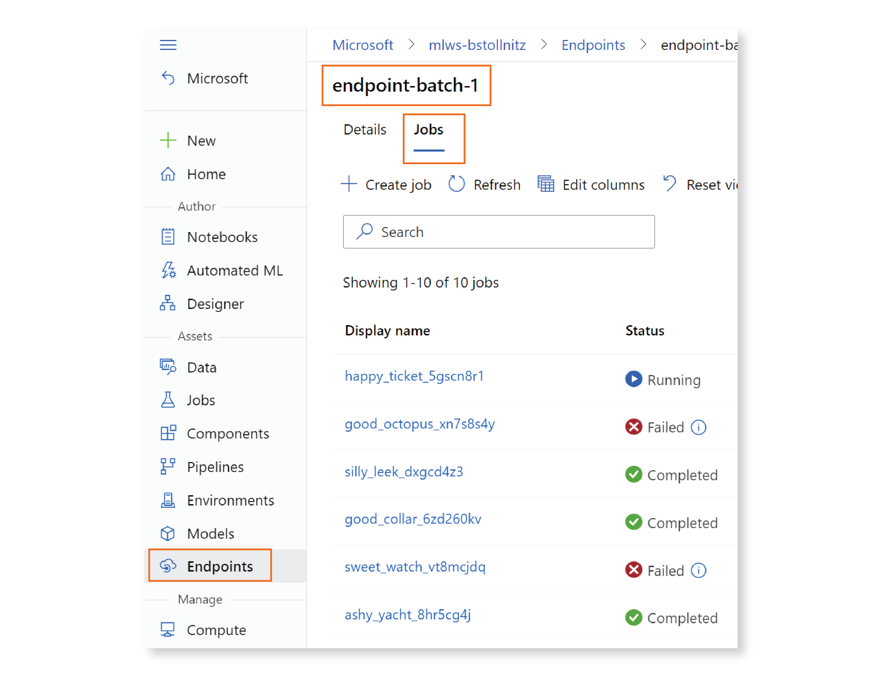
Unlike with managed online endpoints, the invocation call will not immediately return the result of your predictions — instead, it kicks off an asynchronous inference run that will produce predictions at a later time. Let’s go to the Studio and see what’s going on. Click on “Endpoints” in the left navigation, then “Batch endpoints,” and then on the name of your endpoint. You’ll be led to a page with two tabs: “Details,” which shows the information you specified in the endpoint’s YAML file, and “Jobs,” where you can see the status of asynchronous inference job instances associated with the endpoint. Let’s click on “Jobs.” You’ll see all the job instances that were kicked off by the invoke command for this endpoint, with a status that may be “Running,” “Completed,” or “Failed.”

Let’s click on the “Display name” of the latest job. If your job is still running, you can see the logs as they’re generated in real-time by opening the panel on the right and selecting “Outputs + logs.”

When the job completes, you can see the predictions by clicking on the “Show data ouputs” link, and then on the “Access data” icon:

This will take you to the blob storage location where the file containing the predictions is located. If you right-click on the predictions_pytorch.csv file and choose “View/edit,” you’ll see the predictions:

The prediction for each image is a list of 10 values, each representing how likely the image is of containing a particular clothing item. For example, the largest value for image 1 is in index 9, which means that this image likely contains an “Ankle boot.” You can read more about the Fashion MNIST dataset in my blog post that explains ML training with PyTorch. Our model returns this list of 10 values for each image, so that’s what the batch endpoint returns to the user.

At some point, you’ll need to convert each of these lists to the corresponding string that represents the predicted class (e.g. “Ankle boot”). If you’re planning on localizing your app, it makes sense to perform this conversion on the client. You could simply take the argmax of the list returned by the endpoint to get the predicted index, and then convert the index to the corresponding string. But if you’re targeting a single language, it would be more user-friendly to return the text directly from the endpoint. How can we do that? That’s what endpoint 2 is about.

Endpoint 2 - an endpoint with custom code

Endpoint 2 demonstrates how to write custom code that gets executed when the batch endpoint is invoked. MLflow supports this scenario through the creation of a custom model that wraps the original model that we saw in the previous section. This wrapper model must derive from mlflow.pyfunc.PythonModel, and is expected to contain the original model as an artifact, as you can see in the documentation. The wrapper model in model_wrapper.py needs to implement a load_context function that loads the original model from the artifact, and a predict function with the custom prediction code:

import logging

import mlflow
import pandas as pd
import torch

from common import ARTIFACT_NAME

labels_map = {
    0: 'T-Shirt',
    1: 'Trouser',
    2: 'Pullover',
    3: 'Dress',
    4: 'Coat',
    5: 'Sandal',
    6: 'Shirt',
    7: 'Sneaker',
    8: 'Bag',
    9: 'Ankle Boot',
}


class ModelWrapper(mlflow.pyfunc.PythonModel):
    """
    Wrapper for mlflow model.
    """

    def load_context(self, context: mlflow.pyfunc.PythonModelContext) -> None:
        self.model = mlflow.pytorch.load_model(context.artifacts[ARTIFACT_NAME])

    def predict(self, context: mlflow.pyfunc.PythonModelContext,
                model_input: pd.DataFrame) -> list[str]:
        with torch.no_grad():
            device = 'cuda' if torch.cuda.is_available() else 'cpu'
            logging.info('Device: %s', device)

            tensor_input = torch.Tensor(model_input.values).to(device)
            y_prime = self.model(tensor_input)
            probabilities = torch.nn.functional.softmax(y_prime, dim=1)
            predicted_indices = probabilities.argmax(1)
            predicted_names = [
                labels_map[predicted_index.item()]
                for predicted_index in predicted_indices
            ]
        return predicted_names

The code in the predict function calls our model by passing a tensor with pixel values for the input images. The model returns 10 floating point values per image, indicating the likelihood of each clothing item being the right prediction for that image. We then get the index that corresponds to the highest value (using argmax), and get the string that corresponds to that index. The labels_map dictionary shows how to map from indices to strings. So for example, if the largest value appears as the last item on the output list for a particular image, then the prediction for that image is “Ankle boot.”

Notice that the predict function expects the input to be of type DataFrame — this is different from endpoint 1, where the input to our model was a PyTorch tensor. That’s because endpoint 1 gets invoked with images as input, while endpoint 2 receives a CSV file. You can see this information in the documentation, under “File’s types support.”

The CSV file we’ll use as input to the endpoint contains tabular data where each row corresponds to an image, and each column corresponds to a pixel within the image. There are 28 × 28 = 784 pixels in each image, and the column headers have names from “col_0” through “col_783”. Here’s a snippet of the contents of the images.csv file:

col_0,col_1,col_2,col_3,col_4,col_5,col_6,col_7,col_8,col_9,col_10, ... col_783
0.000000,0.000000,0.000000,0.000000,0.000000,0.000000,0.000000,0.000000,0.000000,0.000000, ... 0.000000
0.000000,0.000000,0.000000,0.000000,0.000000,0.000000,0.000000,0.000000,0.000000,0.000000, ... 0.000000
...

You can find the code that generates this CSV file in the generate_images.py file.

Now let’s look at the code that saves the model in train.py:

...
def save_model(pytorch_model_dir: str, pyfunc_model_dir: str,
               model: nn.Module) -> None:
    """
    Saves the trained model.
    """
    # Save PyTorch model.
    pytorch_input_schema = Schema([
        TensorSpec(np.dtype(np.float32), (-1, 784)),
    ])
    pytorch_output_schema = Schema([TensorSpec(np.dtype(np.float32), (-1, 10))])
    pytorch_signature = ModelSignature(inputs=pytorch_input_schema,
                                       outputs=pytorch_output_schema)

    pytorch_code_filenames = ["neural_network.py", "utils_train_nn.py"]
    pytorch_full_code_paths = [
        Path(Path(__file__).parent, code_path)
        for code_path in pytorch_code_filenames
    ]
    logging.info("Saving PyTorch model to %s", pytorch_model_dir)
    shutil.rmtree(pytorch_model_dir, ignore_errors=True)
    mlflow.pytorch.save_model(pytorch_model=model,
                              path=pytorch_model_dir,
                              code_paths=pytorch_full_code_paths,
                              signature=pytorch_signature)

    # Save PyFunc model that wraps the PyTorch model.
    pyfunc_input_schema = Schema(
        [ColSpec(type="double", name=f"col_{i}") for i in range(784)])
    pyfunc_output_schema = Schema([TensorSpec(np.dtype(str), (-1, 1))])
    pyfunc_signature = ModelSignature(inputs=pyfunc_input_schema,
                                      outputs=pyfunc_output_schema)

    pyfunc_code_filenames = ["model_wrapper.py", "common.py"]
    pyfunc_full_code_paths = [
        Path(Path(__file__).parent, code_path)
        for code_path in pyfunc_code_filenames
    ]
    model = ModelWrapper()
    artifacts = {
        ARTIFACT_NAME: pytorch_model_dir,
    }
    conda_env = Path(pytorch_model_dir, "conda.yaml").as_posix()
    logging.info("Saving PyFunc model to %s", pyfunc_model_dir)
    shutil.rmtree(pyfunc_model_dir, ignore_errors=True)
    mlflow.pyfunc.save_model(path=pyfunc_model_dir,
                             python_model=model,
                             artifacts=artifacts,
                             code_path=pyfunc_full_code_paths,
                             conda_env=conda_env,
                             signature=pyfunc_signature)
...

The first part of this code saves the original PyTorch model, and looks exactly like the code for endpoint 1. The second part saves the wrapper model with the custom code. This time our input signature uses a ColSpec instead of a TensorSpec, because we intend to pass a CSV file as input (see the docs). In addition to the type, ColSpec expects a list with the column names in the CSV file, which as we saw earlier range from “col_0” to “col_783”. The output signature is still a TensorSpec, but this time with type str and shape (-1, 1). That’s because our custom code returns a single string classification label for each image.

We save the model wrapper using mlflow.pyfunc.save_model, by giving it all the data we covered in endpoint 1 and two additional pieces of information: a conda file with the packages needed to run our custom code, and the original model stored as an artifact.

To train the model for endpoint 2, select the “Train endpoint 2 locally” run configuration and press F5. This generates two folders, pyfunc_model and pytorch_model. To make a local prediction for this endpoint, we can execute the following command:

cd ../endpoint_2
mlflow models predict --model-uri pyfunc_model --input-path "../test_data/images.csv" --content-type csv

This is very convenient. Since our endpoint expects a CSV file, this time we can use this handy CLI command to test inference locally, instead of writing custom test code. You should get a prediction similar to the following:

["Ankle Boot", "Pullover", "Trouser", "Trouser", "Shirt", "Trouser", "Coat", "Shirt", "Sandal", "Sneaker", "Coat", "Sandal", "Sandal", "Dress", "Coat", "Trouser", "Pullover", "Pullover", "Bag", "T-Shirt"]

Once you’re happy with the predictions you get locally, you’re ready to deploy to the cloud. The process to deploy this endpoint to Azure ML is exactly the same as described for endpoint 1, so I won’t go over it again.

Here’s how you can invoke endpoint 2 using the CLI:

az ml batch-endpoint invoke --name endpoint-batch-2 --input ../test_data/images.csv --input-type uri_file

You can also invoke the endpoint using a POST command. The first step is to register your input data as an asset on Azure ML. Here’s data-invoke-batch.yml, the YAML file containing the details of our data asset:

$schema: https://azuremlschemas.azureedge.net/latest/data.schema.json
name: data-invoke-batch-2
path: "../../test_data/images.csv"
type: uri_file

We specify a schema to get Intellisense during development, a name, the path to the CSV file we want to use as input to the endpoint, and a type. By default the type of a data asset is “uri_folder,” so we need to specify that the type is a “uri_file” because our data consists of a single file. We can create the asset with the following command:

az ml data create -f cloud/data-invoke-batch.yml

You can verify its creation in the “Data” left navigation in the Studio.

Now let’s look at the invoke.sh script that executes a POST request for this endpoint:

ENDPOINT_NAME=endpoint-batch-2
DATASET_NAME=data-invoke-batch-2
DATASET_VERSION=3

SUBSCRIPTION_ID=$(az account show --query id | tr -d '\r"')
echo "SUBSCRIPTION_ID: $SUBSCRIPTION_ID"

RESOURCE_GROUP=$(az group show --query name | tr -d '\r"')
echo "RESOURCE_GROUP: $RESOURCE_GROUP"

WORKSPACE=$(az configure -l | jq -r '.[] | select(.name=="workspace") | .value')
echo "WORKSPACE: $WORKSPACE"

SCORING_URI=$(az ml batch-endpoint show --name $ENDPOINT_NAME --query scoring_uri -o tsv)
echo "SCORING_URI: $SCORING_URI"

SCORING_TOKEN=$(az account get-access-token --resource https://ml.azure.com --query accessToken -o tsv)
echo "SCORING_TOKEN: $SCORING_TOKEN"

curl --location --request POST $SCORING_URI \
--header "Authorization: Bearer $SCORING_TOKEN" \
--header "Content-Type: application/json" \
--data-raw "{
    \"properties\": {
        \"inputData\": {
            \"uriFile\": {
                \"uri\": \"/subscriptions/$SUBSCRIPTION_ID/resourceGroups/$RESOURCE_GROUP/providers/Microsoft.MachineLearningServices/workspaces/$WORKSPACE/data/$DATASET_NAME/versions/$DATASET_VERSION\",
                \"jobInputType\": \"UriFile\"
            }
        },
        \"outputData\": {
            \"uriFile\": {
                \"uri\": \"azureml://datastores/workspaceblobstore/paths/$ENDPOINT_NAME/batch-endpoint-output.csv\",
                \"jobOutputType\": \"UriFile\"
            }
        }
    }
}"

Make sure you change the first three variables to your endpoint name, dataset name, and dataset version. We query for the scoring URI to use as a parameter to the POST command, and we query for the scoring token to use as a bearer token. Then in the --data-raw section, we specify that we want the input to the endpoint to be the data asset we created earlier, and we give it a blob storage location for our output predictions. The type of our input is “UriFile” because our data asset consists of a single file, and similarly for our output. The keys “uriFile” under “inputData” and “outputData” are arbitrary strings.

You can now run this script to invoke the batch endpoint:

chmod +x invoke.sh
./invoke.sh

The first time you run the script, you may have to change the file’s permissions to allow execution. Then you can just execute it in the CLI.

You can look at your predictions by clicking on “Datastores” in the Studio, then “workspaceblobstore,” and then “Browse” in the top navigation (assuming you’re using the same datastore as specified in the script). Alternatively, you can install the Microsoft Azure Storage Explorer. This app provides a nice user interface to manage the files in your datastores, including deleting files.

Conclusion

In this post, you learned how to deploy MLflow models with batch endpoints. You saw how to create a simple endpoint that returns the model’s output as is, and how to create a slightly more advanced endpoint that provides custom code to be executed at inference time.

If you read this post and my blog post on deploying MLflow models with managed online endpoints, you learned about all the supported endpoint input types, and how to test inference locally depending on the type of input. I’ll conclude with a quick summary table of all the MLflow scenarios for you to use as reference.

Thank you for reading, and good luck with your Azure ML projects!

Read next: Creating batch endpoints in Azure ML without using MLflow