Training and deploying your PyTorch model in the cloud with Azure ML
Created:
Topic: Azure ML + PyTorch: better together
Introduction
You’ve been training your PyTorch models on your machine, and getting by just fine. Why would you want to train and deploy them in the cloud? Training in the cloud will allow you to handle larger ML models and datasets than you could train on your development machine. And deploying your model in the cloud will allow your system to scale to many more inference requests than a development machine could handle. In short, moving your code to the cloud will open up a new world of possibilities by scaling up the hard work you’ve already done.
The good news is that moving your PyTorch models to the cloud using Azure ML is fairly straightforward. In this article, I will show you how to train and deploy a simple Fashion MNIST model in the cloud. The steps you’ll see here are the same regardless of the complexity of your PyTorch model, so by the end of this article you’ll be well prepared to apply them to your own work.
You can find the project associated with this post on GitHub, including complete instructions on how to run it.
Step 1: Train and test your PyTorch model locally
You’re probably already done with this step. I added it here anyway because I can’t emphasize enough that your model should be working as expected before you move it to the cloud. You’ll be so much more efficient this way — iterating on code is quick when you do it locally, but a training roundtrip to the cloud takes much longer! If your dataset is too large to train locally, use a portion of your data, and then add the full dataset right before moving to the cloud.
Since we’re using Fashion MNIST, which consists of only 70,000 images, we can train our model locally using the full dataset. If you’re not familiar with the Fashion MNIST dataset and how to write the PyTorch code to train a classifier for this data, you can read this post for more information. Below you can see the training code for our scenario, which can be found in the train.py file of the accompanying GitHub project:
"""Training and evaluation."""

import argparse
import logging
import shutil
from pathlib import Path

import mlflow
import numpy as np
import torch
from mlflow.models.signature import ModelSignature
from mlflow.types.schema import ColSpec, Schema, TensorSpec
from torch import nn
from torch.utils.data import DataLoader, random_split
from torchvision import datasets
from torchvision.transforms import ToTensor

from neural_network import NeuralNetwork
from utils_train_nn import evaluate, fit

DATA_DIR = "aml_command_sdk/data"
MODEL_DIR = "aml_command_sdk/model/"


def load_train_val_data(
    data_dir: str, batch_size: int, training_fraction: float
) -> tuple[DataLoader[torch.Tensor], DataLoader[torch.Tensor]]:
    """
    Returns two DataLoader objects that wrap training and validation data.
    Training and validation data are extracted from the full original training
    data, split according to training_fraction.
    """
    full_train_data = datasets.FashionMNIST(data_dir,
                                            train=True,
                                            download=True,
                                            transform=ToTensor())
    full_train_len = len(full_train_data)
    train_len = int(full_train_len * training_fraction)
    val_len = full_train_len - train_len
    (train_data, val_data) = random_split(dataset=full_train_data,
                                          lengths=[train_len, val_len])
    train_loader = DataLoader(train_data, batch_size=batch_size, shuffle=True)
    val_loader = DataLoader(val_data, batch_size=batch_size, shuffle=True)

    return (train_loader, val_loader)


def save_model(model_dir: str, model: nn.Module) -> None:
    """
    Saves the trained model.
    """
    input_schema = Schema(
        [ColSpec(type="double", name=f"col_{i}") for i in range(784)])
    output_schema = Schema([TensorSpec(np.dtype(np.float32), (-1, 10))])
    signature = ModelSignature(inputs=input_schema, outputs=output_schema)

    code_paths = ["neural_network.py", "utils_train_nn.py"]
    full_code_paths = [
        Path(Path(__file__).parent, code_path) for code_path in code_paths
    ]

    shutil.rmtree(model_dir, ignore_errors=True)
    logging.info("Saving model to %s", model_dir)
    mlflow.pytorch.save_model(pytorch_model=model,
                              path=model_dir,
                              code_paths=full_code_paths,
                              signature=signature)


def train(data_dir: str, model_dir: str, device: str) -> None:
    """
    Trains the model for a number of epochs, and saves it.
    """
    learning_rate = 0.1
    batch_size = 64
    epochs = 5

    (train_dataloader,
     val_dataloader) = load_train_val_data(data_dir, batch_size, 0.8)
    model = NeuralNetwork()
    loss_fn = nn.CrossEntropyLoss()
    optimizer = torch.optim.SGD(model.parameters(), lr=learning_rate)

    for epoch in range(epochs):
        logging.info("Epoch %d", epoch + 1)
        (training_loss, training_accuracy) = fit(device, train_dataloader,
                                                 model, loss_fn, optimizer)
        (validation_loss,
         validation_accuracy) = evaluate(device, val_dataloader, model, loss_fn)

        metrics = {
            "training_loss": training_loss,
            "training_accuracy": training_accuracy,
            "validation_loss": validation_loss,
            "validation_accuracy": validation_accuracy
        }
        mlflow.log_metrics(metrics, step=epoch)

    save_model(model_dir, model)


def main() -> None:
    logging.basicConfig(level=logging.INFO)

    parser = argparse.ArgumentParser()
    parser.add_argument("--data_dir", dest="data_dir", default=DATA_DIR)
    parser.add_argument("--model_dir", dest="model_dir", default=MODEL_DIR)
    args = parser.parse_args()
    logging.info("input parameters: %s", vars(args))

    device = "cuda" if torch.cuda.is_available() else "cpu"

    train(**vars(args), device=device)


if __name__ == "__main__":
    main()
As you can see, we use the MLflow open source framework to save the model and log metrics. Using MLflow is not a requirement when using Azure ML — logging using any other logging framework and saving your model using PyTorch would work perfectly fine. However, MLflow logging displays nicely in Azure ML, and saving a model using the MLflow format simplifies Azure ML deployment, so I’ve been embracing this framework more and more lately.
Our PyTorch neural network can be found in the neural_network.py file of the GitHub project, and it can be seen below:
"""Neural network class."""
import torch
from torch import nn
class NeuralNetwork(nn.Module):
"""
Neural network that classifies Fashion MNIST-style images.
"""
def __init__(self) -> None:
super().__init__()
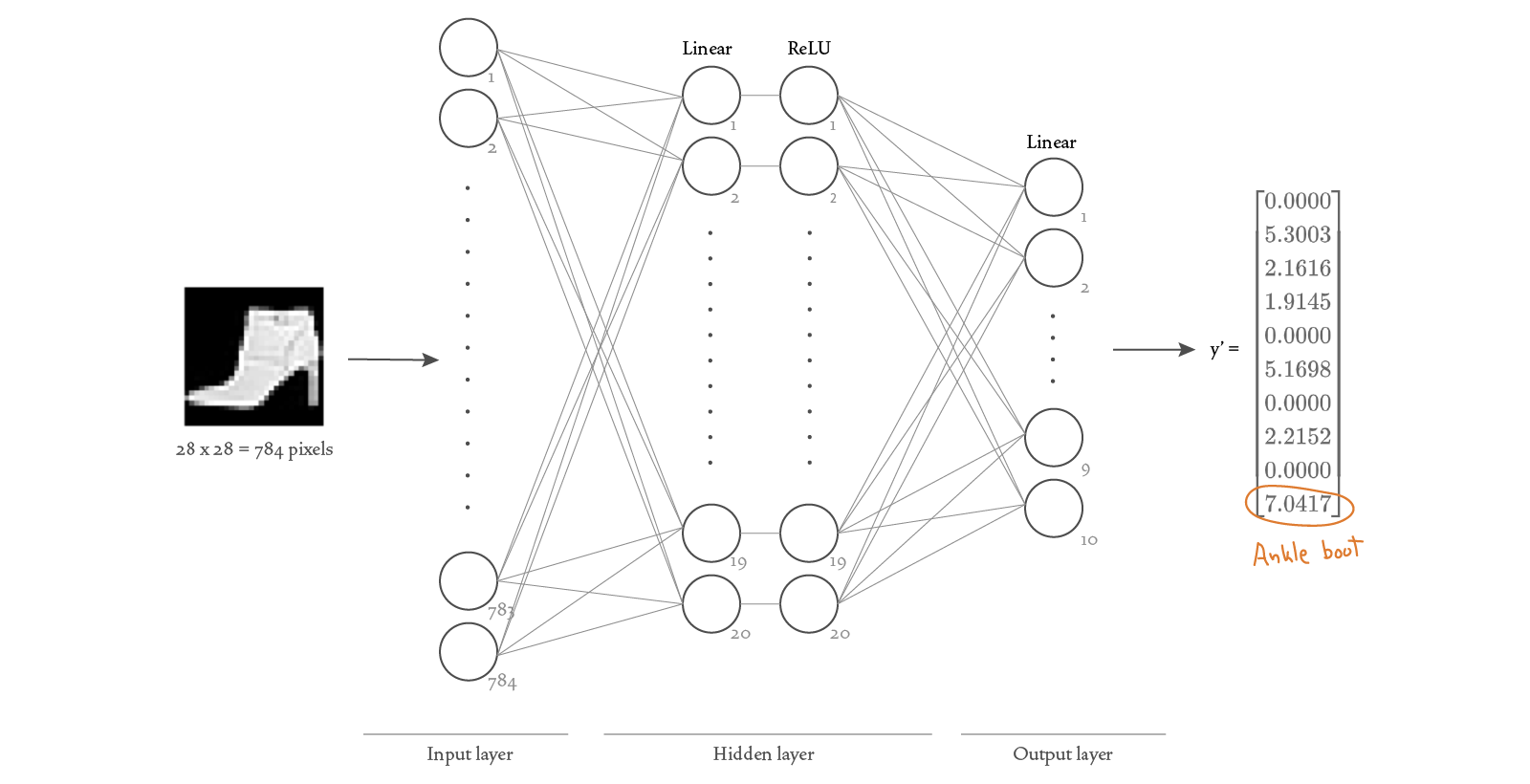
self.sequence = nn.Sequential(nn.Flatten(), nn.Linear(28 * 28, 20),
nn.ReLU(), nn.Linear(20, 10))
def forward(self, x: torch.Tensor) -> torch.Tensor:
y_prime = self.sequence(x)
return y_prime
Our neural network is pretty simple: we have an input layer that takes 28 x 28 pixels as input (the size of a single Fashion MNIST image), a hidden layer with 20 nodes followed by ReLU activation functions, and an output layer with 10 nodes, one for each clothing item. This allows us to input an image of size 28x28, and get back a vector of 10 values, with the highest output value revealing our prediction!
The PyTorch code we use to fit and evaluate our model can be found in the utils_train_nn.py file of our project. Here’s the code:
"""Utilities that help with training neural networks."""

from tqdm import tqdm

import torch
from torch import nn
from torch.nn.modules.loss import CrossEntropyLoss
from torch.optim import Optimizer
from torch.utils.data import DataLoader


def fit(device: str, dataloader: DataLoader[torch.Tensor], model: nn.Module,
        loss_fn: CrossEntropyLoss, optimizer: Optimizer) -> tuple[float, float]:
    """
    Trains the given model for a single epoch.
    """
    loss_sum = 0.0
    correct_item_count = 0
    item_count = 0

    model.to(device)
    model.train()

    for (x, y) in tqdm(dataloader):
        x = x.float().to(device)
        y = y.long().to(device)

        (y_prime, loss) = _fit_one_batch(x, y, model, loss_fn, optimizer)

        correct_item_count += (y_prime.argmax(1) == y).sum().item()
        loss_sum += loss.item()
        item_count += len(x)

    average_loss = loss_sum / item_count
    accuracy = correct_item_count / item_count

    return (average_loss, accuracy)


def _fit_one_batch(x: torch.Tensor, y: torch.Tensor, model: nn.Module,
                   loss_fn: CrossEntropyLoss,
                   optimizer: Optimizer) -> tuple[torch.Tensor, torch.Tensor]:
    """
    Trains a single minibatch (backpropagation algorithm).
    """
    y_prime = model(x)
    loss = loss_fn(y_prime, y)

    optimizer.zero_grad()
    loss.backward()
    optimizer.step()

    return (y_prime, loss)


def evaluate(device: str, dataloader: DataLoader[torch.Tensor],
             model: nn.Module,
             loss_fn: CrossEntropyLoss) -> tuple[float, float]:
    """
    Evaluates the given model for the whole dataset once.
    """
    loss_sum = 0.0
    correct_item_count = 0
    item_count = 0

    model.to(device)
    model.eval()

    with torch.no_grad():
        for (x, y) in dataloader:
            x = x.float().to(device)
            y = y.long().to(device)

            (y_prime, loss) = _evaluate_one_batch(x, y, model, loss_fn)

            correct_item_count += (y_prime.argmax(1) == y).sum().item()
            loss_sum += loss.item()
            item_count += len(x)

        average_loss = loss_sum / item_count
        accuracy = correct_item_count / item_count

    return (average_loss, accuracy)


def _evaluate_one_batch(
        x: torch.Tensor, y: torch.Tensor, model: nn.Module,
        loss_fn: CrossEntropyLoss) -> tuple[torch.Tensor, torch.Tensor]:
    """
    Evaluates a single minibatch.
    """
    with torch.no_grad():
        y_prime = model(x)
        loss = loss_fn(y_prime, y)

    return (y_prime, loss)
This file contains fairly generic PyTorch code to train and evaluate a model, using a concise API. Depending on your scenario, you may be able to reuse it as is, and simply call “fit” to train your model for a single epoch, and “evaluate” to evaluate it. You can look back at the train.py file to see how I use this API.
To train the model you just need to execute the “train.py” file, optionally passing in a path for the data and another path for the model. Since the data is small and the neural network is simple, the model should take just a few minutes to train on your development machine.
You could write some more PyTorch code to test your model. But in this project I decided to use MLflow’s CLI instead, which enables me to test my model without writing any extra code. Here’s the command I execute:
mlflow models predict --model-uri "model" --input-path "test_data/images.json" --content-type json --env-manager local
In this command, “model-uri” refers to the path to our saved model, and “input-path” refers to a file containing the pixel values of two test images. I’m using a JSON file in this case, but MLflow also supports CSV.
You should get predictions for the two images that are similar to the following:
[
  {"0": -3.6867828369140625, "1": -5.797521591186523, "2": -3.2098610401153564, "3": -2.2174417972564697, "4": -2.5920114517211914, "5": 3.298574686050415, "6": -0.4601913094520569, "7": 4.433833599090576, "8": 1.1174960136413574, "9": 5.766951560974121},
  {"0": 3.5685975551605225, "1": -7.8351311683654785, "2": 12.533431053161621, "3": 1.6915751695632935, "4": 6.009798049926758, "5": -6.79791784286499, "6": 7.569240570068359, "7": -6.589715480804443, "8": -2.000182628631592, "9": -8.283203125}
]
Great! You’ve trained and tested your model locally, and are now ready to move your work to the cloud!
Step 2: Train your model in the cloud
In order to train your model in the cloud using Azure ML, you’ll need to create the following Azure ML entities:
- A compute cluster, which specifies the type and number of virtual machines you want to use in the training job.
- A data asset, which contains a copy of your data in the cloud.
- An environment, which specifies the software you’d like to have installed on your virtual machines.
- A command job, which defines the location of your training code together with any inputs and outputs.
The command job uses your compute cluster, data, and environment, and it runs your training code in the cloud. Once it finishes execution, it produces a trained model, which you can register as an Azure ML resource and download locally. You can get a good overview of the entities available in Azure ML in this blog post. The code to create these entities can be found in the job.py file of the current post’s project, or below:
"""Creates and runs an Azure ML command job."""

import logging
from pathlib import Path

from azure.ai.ml import MLClient, Input, Output, command
from azure.ai.ml.constants import AssetTypes
from azure.identity import DefaultAzureCredential
from azure.ai.ml.entities import (AmlCompute, Data, Environment, Model)

from common import MODEL_NAME

COMPUTE_NAME = "cluster-cpu"
DATA_NAME = "data-fashion-mnist"
DATA_PATH = Path(Path(__file__).parent.parent, "data")
CONDA_PATH = Path(Path(__file__).parent, "conda.yml")
CODE_PATH = Path(Path(__file__).parent.parent, "src")
MODEL_PATH = Path(Path(__file__).parent.parent)


def main() -> None:
    logging.basicConfig(level=logging.INFO)
    credential = DefaultAzureCredential()
    ml_client = MLClient.from_config(credential=credential)

    # Create the compute cluster.
    cluster_cpu = AmlCompute(
        name=COMPUTE_NAME,
        type="amlcompute",
        size="Standard_DS4_v2",
        location="westus2",
        min_instances=0,
        max_instances=4,
    )
    ml_client.begin_create_or_update(cluster_cpu)

    # Create the data set.
    dataset = Data(
        name=DATA_NAME,
        description="Fashion MNIST data set",
        path=DATA_PATH.as_posix(),
        type=AssetTypes.URI_FOLDER,
    )
    ml_client.data.create_or_update(dataset)

    # Create the environment.
    environment = Environment(image="mcr.microsoft.com/azureml/" +
                              "openmpi4.1.0-ubuntu20.04:latest",
                              conda_file=CONDA_PATH)

    # Create the job.
    job = command(
        description="Trains a simple neural network on the Fashion-MNIST " +
        "dataset.",
        experiment_name="aml_command_sdk",
        compute=COMPUTE_NAME,
        inputs=dict(fashion_mnist=Input(path=f"{DATA_NAME}@latest")),
        outputs=dict(model=Output(type=AssetTypes.MLFLOW_MODEL)),
        code=CODE_PATH,
        environment=environment,
        command="python train.py --data_dir ${{inputs.fashion_mnist}} " +
        "--model_dir ${{outputs.model}}",
    )
    job = ml_client.jobs.create_or_update(job)
    ml_client.jobs.stream(job.name)

    # Create the model.
    model_path = f"azureml://jobs/{job.name}/outputs/model"
    model = Model(name=MODEL_NAME,
                  path=model_path,
                  type=AssetTypes.MLFLOW_MODEL)
    registered_model = ml_client.models.create_or_update(model)

    # Download the model (this is optional).
    ml_client.models.download(name=MODEL_NAME,
                              download_path=MODEL_PATH,
                              version=registered_model.version)


if __name__ == "__main__":
    main()
There are actually three different ways for creating these resources: from your terminal using the Azure ML CLI and YAML configuration files which I cover in this post, with a low-code approach using the Azure ML studio, or by writing code using the Azure ML Python SDK, which is the method I show in our current post. Regardless of which option you choose, you can visualize the results of your work in the Azure ML studio. From the left navigation pane of the studio, you can click on “Compute,” “Data,” “Environments,” “Jobs,” and “Model” to see the entities you just created!
Step 3: Deploy your model to the cloud
Now that you have a trained model registered in the cloud, let’s look at how you can deploy it. This will enable you and your users to make a prediction using the trained model from anywhere, at scale. In order to deploy with Azure ML, we’ll need to create the following two resources:
- A Managed Online Endpoint, which is one of a few different types of endpoints supported by Azure ML. We’ll use this particular endpoint for this scenario because it’s designed to process smaller requests and give near-immediate responses.
- A Managed Online Deployment, which contains information about the trained model and compute we want to use. Our endpoint can accommodate more than one deployment, but we’ll use just one in our simple scenario.
The code that creates these resources can be found on the endpoint.py file of the accompanying project. You can also see it below:
"""Creates and invokes a managed online endpoint."""

import logging
from pathlib import Path

from azure.ai.ml import MLClient
from azure.ai.ml.entities import ManagedOnlineDeployment, ManagedOnlineEndpoint
from azure.identity import DefaultAzureCredential

from common import MODEL_NAME, ENDPOINT_NAME

DEPLOYMENT_NAME = "blue"
TEST_DATA_PATH = Path(
    Path(__file__).parent.parent, "test_data", "images_azureml.json")


def main() -> None:
    logging.basicConfig(level=logging.INFO)
    credential = DefaultAzureCredential()
    ml_client = MLClient.from_config(credential=credential)

    # Create the managed online endpoint.
    endpoint = ManagedOnlineEndpoint(
        name=ENDPOINT_NAME,
        auth_mode="key",
    )
    registered_endpoint = ml_client.online_endpoints.begin_create_or_update(
        endpoint).result()

    # Get the latest version of the registered model.
    registered_model = ml_client.models.get(name=MODEL_NAME, label="latest")

    # Create the managed online deployment.
    deployment = ManagedOnlineDeployment(name=DEPLOYMENT_NAME,
                                         endpoint_name=ENDPOINT_NAME,
                                         model=registered_model,
                                         instance_type="Standard_DS4_v2",
                                         instance_count=1)
    ml_client.online_deployments.begin_create_or_update(deployment).result()

    # Set deployment traffic to 100%.
    registered_endpoint.traffic = {"blue": 100}
    ml_client.online_endpoints.begin_create_or_update(
        registered_endpoint).result()

    # Invoke the endpoint.
    result = ml_client.online_endpoints.invoke(endpoint_name=ENDPOINT_NAME,
                                               request_file=TEST_DATA_PATH)
    logging.info(result)


if __name__ == "__main__":
    main()
This code creates the endpoint and deployment, and invokes the endpoint by using a JSON file with Fashion MNIST images as input. You should obtain a prediction similar to what you saw locally.
Before you set your work aside, remember to delete your endpoint if you’re not planning on using it, to avoid getting charged. You can do this by running the delete_endpoint.py file in the project, or by going to the “Endpoints” section in the Azure ML Studio.
And that’s all there is to it! You now have the knowledge you need to train and deploy your machine learning models at scale, in the cloud! :)