Going beyond Keras - customizing with TensorFlow
Created:
Updated:
Topic: Deep learning frameworks
Introduction
Microsoft recently announced a “Going beyond Keras - customizing with TensorFlow” learning module, which my team and I created, covering TensorFlow concepts. You can engage with the tutorial in a notebook-like experience on Microsoft’s site. Or you can read about the same concepts in a more linear format in this post. This is the third part of a series of posts, where I present PyTorch, TensorFlow’s higher-level Keras API, and lower-level concepts of TensorFlow, followed by a comparison between the three. The code for this post can be found on GitHub.
In order to follow this post, I recommend that you first read my Introduction to TensorFlow using Keras blog post, or that you have a solid knowledge of Keras. In the Keras post I show how to create a basic neural network that classifies items of clothing, using the Fashion MNIST dataset as a data source. Keras provides users with a high-level API, which enables us to train, test, and predict with very little code. For those scenarios where you need a little extra control over the flow of your code or network architecture, then TensorFlow is your friend. You’ll need to learn a few extra concepts, and write a bit more code, but you’ll gain endless flexibility in return. In this post, I will show you how to re-implement the model, training and prediction portions of the code in my Keras post, this time using TensorFlow.
Tensors and variables
Before we start re-implementing portions of the Keras code, we need to understand TensorFlow’s basic concepts. In this section, we’ll cover tensors and variables.
In TensorFlow, a Tensor is the data structure used to store the inputs and outputs of a deep learning model. A Variable is a special type of tensor that is used to store any model parameters that need to be learned during training. The difference here is that tensors are immutable and variables are mutable. They’re both super important concepts to understand if you’re going to be working with TensorFlow.
Mathematically speaking, a tensor is just a generalization of vectors and matrices. A vector is a one-dimensional array of values, a matrix is a two-dimensional array of values, and a tensor is an array of values with any number of dimensions. A TensorFlow Tensor, much like NumPy’s ndarray, gives us a way to represent multidimensional data, but with added tricks, such as the ability to perform operations on a GPU and the ability to calculate derivatives.
Suppose we want to represent this 3 × 2 matrix in TensorFlow:
Here’s the code to create the corresponding tensor:
X = tf.constant([[1, 2], [3, 4], [5, 6]])
We can inspect the tensor’s shape attribute to see how many dimensions it has and the size in each dimension. The device attribute tells us whether the tensor is stored on the CPU or GPU, and the dtype attribute indicates what kind of values it holds. We use the type function to check the type of the tensor itself.
print(X.shape)
print(X.device)
print(X.dtype)
print(type(X))
(3, 2)
/job:localhost/replica:0/task:0/device:CPU:0
<dtype: 'int32'>
<class 'tensorflow.python.framework.ops.EagerTensor'>
Note that if your machine is configured properly for TensorFlow to take advantage of a GPU, then TensorFlow will automatically decide whether to store tensors and perform tensor math on the GPU or CPU in an optimal way, without any additional work on your part.
If you’ve used NumPy ndarrays before, you might be happy to know that TensorFlow tensors can be indexed in a familiar way. We can slice a tensor to view a smaller portion of it:
X = X[0:2, 0:1]
print(X)
<tf.Tensor: shape=(2, 1), dtype=int32, numpy=
array([[1],
       [3]], dtype=int32)>
We can also convert tensors to NumPy arrays by simply using the numpy method:
array = X.numpy()
print(array)
array([[1],
       [3]], dtype=int32)
Variables can easily be initialized from tensors:
V = tf.Variable(X)
print(V)
<tf.Variable 'Variable:0' shape=(2, 1) dtype=int32, numpy=
array([[1],
       [3]], dtype=int32)>
As we mentioned earlier, unlike a Tensor, a Variable is mutable. We can update the value of our variable using the assign, assign_add, and assign_sub methods:
Y = tf.constant([[5], [6]])
V.assign(Y)
print(V)
<tf.Variable 'Variable:0' shape=(2, 1) dtype=int32, numpy=
array([[5],
       [6]], dtype=int32)>
V.assign_add([[1], [1]])
print(V)
<tf.Variable 'UnreadVariable' shape=(2, 1) dtype=int32, numpy=
array([[6],
       [7]], dtype=int32)>
V.assign_sub([[2], [2]])
<tf.Variable 'UnreadVariable' shape=(2, 1) dtype=int32, numpy=
array([[4],
       [5]], dtype=int32)>
Automatic differentiation
Part of the machine learning training process requires calculating derivatives that involve tensors. So let’s learn about TensorFlow’s built-in automatic differentiation engine, using a very simple example. Let’s consider the following two tensors:
Now let’s suppose that we want to multiply
Our goal is to calculate the derivative of
# Decimal points in tensor values ensure they are floats, which automatic differentiation requires.
U = tf.constant([[1., 2.]])
V = tf.constant([[3., 4.], [5., 6.]])

with tf.GradientTape(persistent=True) as tape:
  tape.watch(U)
  tape.watch(V)
  W = tf.matmul(U, V)
  f = tf.math.reduce_sum(W)

print(tape.gradient(f, U)) # df/dU
print(tape.gradient(f, V)) # df/dV
tf.Tensor([[ 7. 11.]], shape=(1, 2), dtype=float32)
tf.Tensor(
[[1. 1.]
 [2. 2.]], shape=(2, 2), dtype=float32)
TensorFlow automatically watches tensors that are defined as Variable instances. So let’s turn U and V into variables, and remove the watch calls:
# Decimal points in tensor values ensure they are floats, which automatic differentiation requires.
U = tf.Variable(tf.constant([[1., 2.]]))
V = tf.Variable(tf.constant([[3., 4.], [5., 6.]]))

with tf.GradientTape(persistent=True) as tape:
  W = tf.matmul(U, V)
  f = tf.math.reduce_sum(W)

print(tape.gradient(f, U)) # df/dU
print(tape.gradient(f, V)) # df/dV
tf.Tensor([[ 7. 11.]], shape=(1, 2), dtype=float32)
tf.Tensor(
[[1. 1.]
 [2. 2.]], shape=(2, 2), dtype=float32)
As you will see later, in deep learning, we will need to calculate the derivatives of the loss function with respect to the model parameters. Those parameters are variables because they change during training. Therefore, the fact that variables are automatically watched is handy in our scenario.
Let’s take a look at the math used to compute the derivatives. You only need to understand matrix multiplication and partial derivatives to follow along, but if the math isn’t as interesting to you, feel free to skip to the next section.
We’ll start by thinking of
Then the scalar function
We can now calculate the derivatives of
As you can see, when we plug in the numerical values of
The neural network architecture
Now that you’ve learned about tensors, variables, and automatic differentiation, you’re ready to learn how to define a neural network from scratch using lower-level TensorFlow operations. It’s important to understand these foundational concepts because they give you the flexibility to customize your neural networks in any way you like.
As a reminder, here’s the structure of the neural network we defined using Keras:
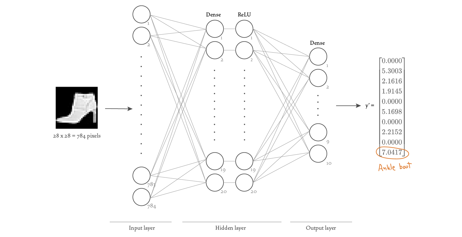
And here’s the same neural network, this time showing the
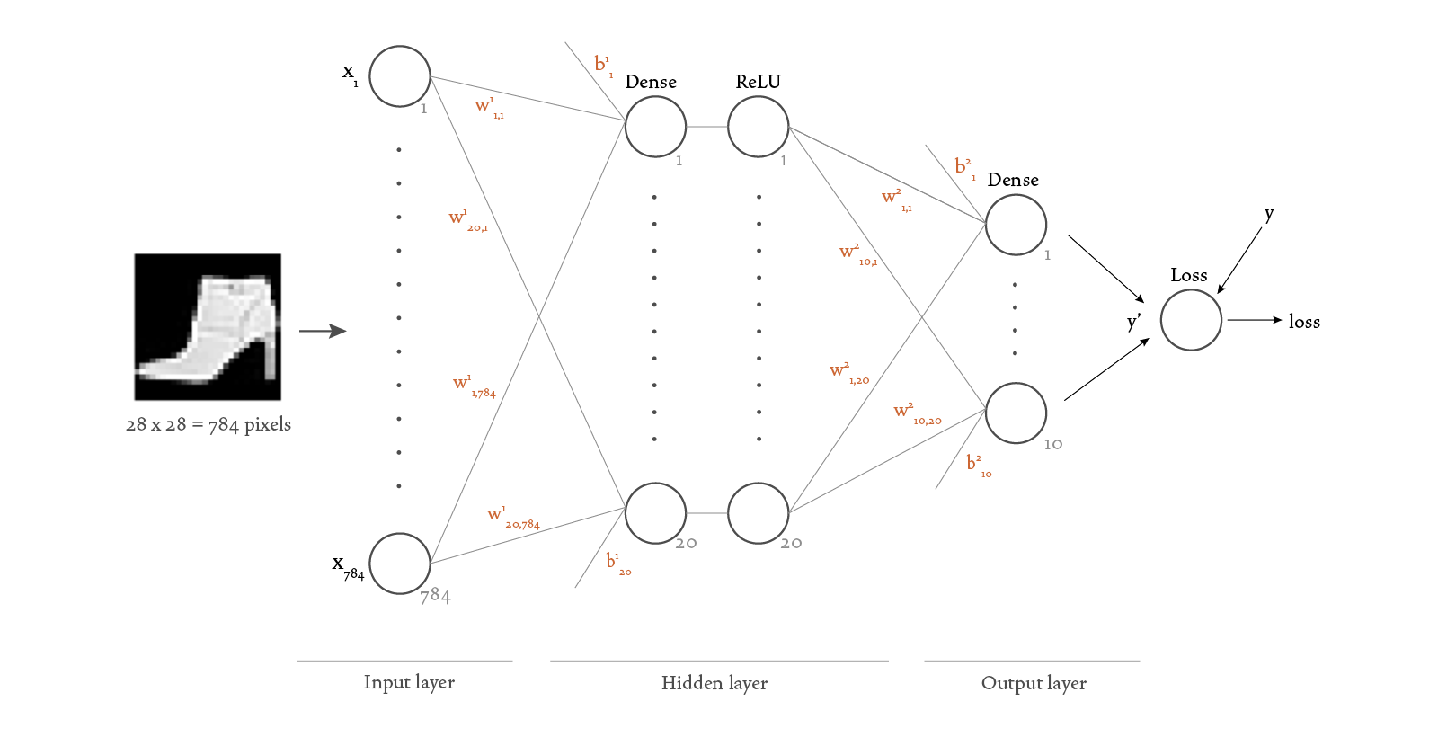
Notice that our neural network is composed of two Dense layers, and that the first of those contains a ReLU (“Rectified Linear Unit”) activation function. In Keras, we can build our model by simply initializing the Dense objects with the appropriate activation functions. If we don’t want to use Keras, we need to understand the operations performed by a Dense layer a bit better and replicate them. It turns out that a Dense layer is just about the simplest type of layer we can use, so it’s not that hard to understand and replicate. A Dense layer takes as input a
The output of the first Dense layer is then passed as input to a ReLU non-linear function in the following way:
Let’s now see how we can represent these concepts using TensorFlow code.
https://github.com/bstollnitz/fashion-mnist-tf/blob/main/fashion-mnist-tf/local-tf/src/neural_network.py
import tensorflow as tf

class NeuralNetwork(tf.keras.Model):
    """Neural network that classifies Fashion MNIST-style images."""

    def __init__(self):
        super().__init__()
        initializer = tf.keras.initializers.GlorotUniform()
        self.w1 = tf.Variable(initializer(shape=(784, 20)))
        self.b1 = tf.Variable(tf.zeros(shape=(20,)))
        self.w2 = tf.Variable(initializer(shape=(20, 10)))
        self.b2 = tf.Variable(tf.zeros(shape=(10,)))

    def call(self, x: tf.Tensor) -> tf.Tensor:
        x = tf.reshape(x, [-1, 784])
        x = tf.matmul(x, self.w1) + self.b1
        x = tf.nn.relu(x)
        x = tf.matmul(x, self.w2) + self.b2
        return x
Notice that here we’re explicitly instantiating parameters Variables (rather than Tensors) because their values change during training. Notice also how we initialize their values — the parameters
Other than that, you can see that the additions, multiplications, and ReLU calls we discussed earlier are reflected in the code as you might expect.
Training the network
Let’s first get the imports for the code in the main.py file, which contains most of the code in this blog post.
https://github.com/bstollnitz/fashion-mnist-tf/blob/main/fashion-mnist-tf/local-tf/src/main.py
import os
import time
from typing import Tuple

os.environ['TF_CPP_MIN_LOG_LEVEL'] = '3'

import numpy as np
import tensorflow as tf
from PIL import Image

from neural_network import NeuralNetwork
You’ve already seen how to train a neural network using Keras in my Introduction to TensorFlow using Keras post — in this post, we’ll re-implement the training loop in TensorFlow. This will help you understand what goes on under the hood a bit better, and will give you the opportunity to customize the training loop if you want.
As I mentioned in the Keras post, the goal of training the neural network is to find parameters
Let’s now dig deeper into what this optimization algorithm might look like. There are many types of optimization algorithms, but in this tutorial we’ll cover only the simplest one: the gradient descent algorithm. To implement gradient descent, we iteratively improve our estimates of
The parameter
When doing training, we pass a mini-batch of data as input, perform a sequence of calculations to obtain the loss, then propagate back through the network to calculate the derivatives used in the gradient descent formulas above. Once we have the derivatives, we can update the values of the network’s parameters
In Keras, when we called the function fit, the backpropagation algorithm was executed several times. Here, we’ll start by understanding the code that reflects a single pass of the backpropagation algorithm:
- a forward pass through the model to compute the predicted value,
y_prime = model(X, training=True) - a calculation of the loss using a loss function,
loss = loss_fn(y, y_prime) - a backward pass from the loss function through the model to calculate derivatives,
grads = tape.gradient(loss, model.trainable_variables) - a gradient descent step to update
and using the derivatives calculated in the backward pass, optimizer.apply_gradients(zip(grads, model.trainable_variables))
Here’s the complete code:
https://github.com/bstollnitz/fashion-mnist-tf/blob/main/fashion-mnist-tf/local-tf/src/main.py
...
def _fit_one_batch(
        x: tf.Tensor, y: tf.Tensor, model: tf.keras.Model,
        loss_fn: tf.keras.losses.Loss, optimizer: tf.keras.optimizers.Optimizer
) -> Tuple[tf.Tensor, tf.Tensor]:
    """Trains a single minibatch (backpropagation algorithm)."""
    with tf.GradientTape() as tape:
        y_prime = model(x, training=True)
        loss = loss_fn(y, y_prime)

    grads = tape.gradient(loss, model.trainable_variables)
    optimizer.apply_gradients(zip(grads, model.trainable_variables))

    return (y_prime, loss)
...
Notice that the code above ensures that the forward calculations are within the GradientTape’s scope, just as we saw in the previous section. This makes it possible for us to ask the tape for the gradients.
The code above works for a single mini-batch, which is typically much smaller than the full set of data (in this sample we use a mini-batch of size 64, out of 60,000 training data items). But we want to execute the backpropagation algorithm for the full set of data. We can do so by iterating through the Dataset we created earlier, which, as we saw in the Keras post, returns a mini-batch per iteration.
Let’s take a look at the code that calls the backpropagation algorithm for all mini-batches in the dataset:
https://github.com/bstollnitz/fashion-mnist-tf/blob/main/fashion-mnist-tf/local-tf/src/main.py
...
def _fit(dataset: tf.data.Dataset, model: tf.keras.Model,
         loss_fn: tf.keras.losses.Loss,
         optimizer: tf.optimizers.Optimizer) -> Tuple[float, float]:
    """Trains the given model for a single epoch."""
    loss_sum = 0
    correct_item_count = 0
    item_count = 0

    # Used for printing only.
    batch_count = len(dataset)
    print_every = 100

    for batch_index, (x, y) in enumerate(dataset):
        x = tf.cast(x, tf.float64)
        y = tf.cast(y, tf.int64)

        (y_prime, loss) = _fit_one_batch(x, y, model, loss_fn, optimizer)

        correct_item_count += (tf.math.argmax(y_prime,
                                              axis=1) == y).numpy().sum()
        loss_sum += loss.numpy()
        item_count += len(x)

        # Printing progress.
        if ((batch_index + 1) % print_every == 0) or ((batch_index + 1)
                                                      == batch_count):
            accuracy = correct_item_count / item_count
            average_loss = loss_sum / item_count
            print(f'[Batch {batch_index + 1:>3d} - {item_count:>5d} items] ' +
                  f'loss: {average_loss:>7f}, ' +
                  f'accuracy: {accuracy*100:>0.1f}%')

    average_loss = loss_sum / item_count
    accuracy = correct_item_count / item_count

    return (average_loss, accuracy)
...
A complete iteration over all mini-batches in the dataset is called an “epoch.” In this sample, we restrict the code to just five epochs for quick execution, but in a real project you would want to set it to a much higher number (to achieve better predictions). The code below also shows the creation of the loss function and optimizer, which we discussed in the Keras post.
https://github.com/bstollnitz/fashion-mnist-tf/blob/main/fashion-mnist-tf/local-tf/src/main.py
...
MODEL_DIRPATH = 'fashion-mnist-tf/local-tf/model/weights'

...

def training_phase():
    """Trains the model for a number of epochs, and saves it."""
    learning_rate = 0.1
    batch_size = 64
    epochs = 5

    (train_dataset, test_dataset) = _get_data(batch_size)

    model = NeuralNetwork()

    loss_fn = tf.keras.losses.SparseCategoricalCrossentropy(from_logits=True)
    optimizer = tf.optimizers.SGD(learning_rate)

    print('\n***Training***')

    for epoch in range(epochs):
        print(f'\nEpoch {epoch + 1}\n-------------------------------')
        (train_loss, train_accuracy) = _fit(train_dataset, model, loss_fn,
                                            optimizer)
        print(f'Train loss: {train_loss:>8f}, ' +
              f'train accuracy: {train_accuracy * 100:>0.1f}%')

    print('\n***Evaluating***')
    (test_loss, test_accuracy) = _evaluate(test_dataset, model, loss_fn)
    print(f'Test loss: {test_loss:>8f}, ' +
          f'test accuracy: {test_accuracy * 100:>0.1f}%')

    model.save_weights(MODEL_DIRPATH)
...
***Training***

Epoch 1
-------------------------------
[Batch 100 -  6400 items] accuracy: 53.0%, loss: 0.666479
[Batch 200 - 12800 items] accuracy: 63.9%, loss: 0.961517
[Batch 300 - 19200 items] accuracy: 67.8%, loss: 0.634329
[Batch 400 - 25600 items] accuracy: 70.3%, loss: 0.559344
[Batch 500 - 32000 items] accuracy: 72.0%, loss: 0.411280
[Batch 600 - 38368 items] accuracy: 73.4%, loss: 0.355198
[Batch 700 - 44768 items] accuracy: 74.4%, loss: 0.522750
[Batch 800 - 51168 items] accuracy: 75.2%, loss: 0.452843
[Batch 900 - 57568 items] accuracy: 75.9%, loss: 0.634226
[Batch 938 - 60000 items] accuracy: 76.1%, loss: 0.446549

...

Epoch 5
-------------------------------
[Batch 100 -  6400 items] accuracy: 85.0%, loss: 0.433118
[Batch 200 - 12800 items] accuracy: 85.3%, loss: 0.327807
[Batch 300 - 19200 items] accuracy: 85.4%, loss: 0.382435
[Batch 400 - 25600 items] accuracy: 85.5%, loss: 0.620741
[Batch 500 - 32000 items] accuracy: 85.4%, loss: 0.266501
[Batch 600 - 38400 items] accuracy: 85.5%, loss: 0.427130
[Batch 700 - 44768 items] accuracy: 85.5%, loss: 0.417475
[Batch 800 - 51168 items] accuracy: 85.6%, loss: 0.357484
[Batch 900 - 57568 items] accuracy: 85.6%, loss: 0.407143
[Batch 938 - 60000 items] accuracy: 85.7%, loss: 0.402664
Eager execution and graph execution
Up until now, we’ve been running our code in ”eager execution” mode, which is enabled by default. In this mode, the flow of code execution happens in the order we’re accustomed to, and we can add breakpoints and inspect the values of our tensors and variables as usual.
In contrast, when in ”graph execution” mode, the code execution flows a bit differently: during the first pass through the code, a graph is created containing information about the operations and tensors in that code. Then in subsequent passes, the graph is used instead of the Python code. One consequence of this flow is that our code is not debuggable in the usual manner. We gain two major advantages though:
- The graph can be deployed to environments that don’t have Python, such as embedded devices.
- The graph can take advantage of several performance optimizations, such as running parts of the code in parallel.
In order to get the best of both worlds, we use eager execution mode during the development phase, and then switch to graph execution mode once we’re done debugging the model. To switch from eager to graph execution, we can add the @tf.function decorator to the function containing our model operations.
With that in mind, now that we’re done with development, let’s add the @tf.function decorator to the _fit_one_batch(...) function, which is where we have all the model operations.
https://github.com/bstollnitz/fashion-mnist-tf/blob/main/fashion-mnist-tf/local-tf/src/main.py
...
@tf.function
def _fit_one_batch(
        x: tf.Tensor, y: tf.Tensor, model: tf.keras.Model,
        loss_fn: tf.keras.losses.Loss, optimizer: tf.keras.optimizers.Optimizer
) -> Tuple[tf.Tensor, tf.Tensor]:
    """Trains a single minibatch (backpropagation algorithm)."""
    with tf.GradientTape() as tape:
        y_prime = model(x, training=True)
        loss = loss_fn(y, y_prime)

    grads = tape.gradient(loss, model.trainable_variables)
    optimizer.apply_gradients(zip(grads, model.trainable_variables))

    return (y_prime, loss)
...
Let’s also add a timer to the training_phase() function, so that we can check how long it takes to run training, with and without the @tf.function decorator.
https://github.com/bstollnitz/fashion-mnist-tf/blob/main/fashion-mnist-tf/local-tf/src/main.py
...
def training_phase():
    """Trains the model for a number of epochs, and saves it."""
    learning_rate = 0.1
    batch_size = 64
    epochs = 5

    (train_dataset, test_dataset) = _get_data(batch_size)

    model = NeuralNetwork()

    loss_fn = tf.keras.losses.SparseCategoricalCrossentropy(from_logits=True)
    optimizer = tf.optimizers.SGD(learning_rate)

    print('\n***Training***')
    t_begin = time.time()

    for epoch in range(epochs):
        print(f'\nEpoch {epoch + 1}\n-------------------------------')
        (train_loss, train_accuracy) = _fit(train_dataset, model, loss_fn,
                                            optimizer)
        print(f'Train loss: {train_loss:>8f}, ' +
              f'train accuracy: {train_accuracy * 100:>0.1f}%')

    t_elapsed = time.time() - t_begin
    print(f'\nTime per epoch: {t_elapsed / epochs :>.3f} sec')

    print('\n***Evaluating***')
    (test_loss, test_accuracy) = _evaluate(test_dataset, model, loss_fn)
    print(f'Test loss: {test_loss:>8f}, ' +
          f'test accuracy: {test_accuracy * 100:>0.1f}%')

    model.save_weights(MODEL_DIRPATH)
...
On my machine, eager execution takes more than twice the amount of time to train, compared to graph execution.
Testing the network
Now that we’ve trained our model, we’re ready to test it, which we can do by running a single pass forward through the network. The function _evaluate_one_batch(...) contains the code that does this: we simply need to call the model to get a prediction, followed by the loss function loss_fn to get a score for how the predicted labels y_prime compare to the actual labels y. Notice that we don’t add a tf.GradientTape() this time — that’s because, since we don’t do a backward pass during testing, we don’t need to calculate derivatives for gradient descent. Notice also that we added a @tf.function decorator once we were done with development and debugging, to get a performance boost.
https://github.com/bstollnitz/fashion-mnist-tf/blob/main/fashion-mnist-tf/local-tf/src/main.py
...
@tf.function
def _evaluate_one_batch(
        x: tf.Tensor, y: tf.Tensor, model: tf.keras.Model,
        loss_fn: tf.keras.losses.Loss) -> Tuple[tf.Tensor, tf.Tensor]:
    """Evaluates a single minibatch."""
    y_prime = model(x, training=False)
    loss = loss_fn(y, y_prime)

    return (y_prime, loss)
...
The _evaluate(...) function calls the _evaluate_one_batch(...) function for the entire dataset, once per mini-batch.
https://github.com/bstollnitz/fashion-mnist-tf/blob/main/fashion-mnist-tf/local-tf/src/main.py
...
def _evaluate(dataset: tf.data.Dataset, model: tf.keras.Model,
              loss_fn: tf.keras.losses.Loss) -> Tuple[float, float]:
    """Evaluates the given model for the whole dataset once."""
    loss_sum = 0
    correct_item_count = 0
    item_count = 0

    for (x, y) in dataset:
        x = tf.cast(x, tf.float64)
        y = tf.cast(y, tf.int64)

        (y_prime, loss) = _evaluate_one_batch(x, y, model, loss_fn)

        correct_item_count += (tf.math.argmax(
            y_prime, axis=1).numpy() == y.numpy()).sum()
        loss_sum += loss.numpy()
        item_count += len(x)

    average_loss = loss_sum / item_count
    accuracy = correct_item_count / item_count
    return (average_loss, accuracy)
...
We’ll repeat below the code that calls the _evaluate(...) function, which you already saw earlier as part of the training_phase(...) function.
https://github.com/bstollnitz/fashion-mnist-tf/blob/main/fashion-mnist-tf/local-tf/src/main.py
    ...
    (test_loss, test_accuracy) = _evaluate(test_dataset, model, loss_fn)
    ...
When you run the code above, you’ll see output similar to the following:
***Evaluating***
Test accuracy: 86.0%, test loss: 0.387400
Hopefully the test loss and accuracy you obtained are similar to the training loss and accuracy you obtained earlier. In this case they should be, but if that’s not the case in your future projects, you may need to adjust your data or model.
Making predictions
In order to make a prediction, we need to pass some data to the model, and do a single forward pass through the network to get the prediction. Remember that, unlike during testing, we don’t need to call the loss function because we’re no longer interested in evaluating how well the model is doing. Instead, we call softmax to convert the values of the output vector into values between 0 and 1, and then get the argmax of that vector to get the predicted label index.
Similarly to the training and testing sections, once we’re done with debugging, we can add a @tf.function decorator to get the performance benefits of graph execution.
https://github.com/bstollnitz/fashion-mnist-tf/blob/main/fashion-mnist-tf/local-tf/src/main.py
...
@tf.function
def _predict(model: tf.keras.Model, x: np.ndarray) -> tf.Tensor:
    """Makes a prediction for input x."""
    y_prime = model(x, training=False)
    probabilities = tf.nn.softmax(y_prime, axis=1)
    predicted_indices = tf.math.argmax(input=probabilities, axis=1)
    return predicted_indices
...
In our scenario, we’ll predict the label for the following image:

In the code below, we load the image, call _predict(...) to get its class index, and map that index to the class name.
https://github.com/bstollnitz/fashion-mnist-tf/blob/main/fashion-mnist-tf/local-tf/src/main.py
...
MODEL_DIRPATH = 'fashion-mnist-tf/local-tf/model/weights'
IMAGE_FILEPATH = 'fashion-mnist-tf/local-tf/src/predict-image.png'

...

def inference_phase():
    """Makes a prediction for a local image."""
    print('\n***Predicting***')

    model = NeuralNetwork()
    model.load_weights(MODEL_DIRPATH)

    with Image.open(IMAGE_FILEPATH) as image:
        x = np.asarray(image).reshape((-1, 28, 28)) / 255.0

    predicted_index = _predict(model, x).numpy()[0]
    predicted_name = labels_map[predicted_index]

    print(f'Predicted class: {predicted_name}')
...
***Predicting***
Predicted class: Ankle Boot
Summary
In this blog post, you learned about basic TensorFlow concepts such as tensors, variables, automatic differentiation, eager execution, and graph execution. You then used those concepts to re-implement the model, training, testing, and prediction code from my earlier Keras post, but this time at a lower level, using TensorFlow. You’re now prepared to customize your code in case you ever need more flexibility than Keras offers.
The complete code for this post can be found on GitHub.
Thank you to Dmitry Soshnikov from Microsoft for reviewing the content in this post.