Bea Stollnitz - Introduction to TensorFlow using Keras

Introduction

Microsoft recently released an “Introduction to TensorFlow using Keras” tutorial, which my team and I created, covering both Keras and TensorFlow concepts. You can engage with the tutorial in a notebook-like experience on Microsoft’s site. Or you can read about the same concepts in a more linear format in this post. This is the second part of a series of posts, where I present PyTorch, higher-level TensorFlow using Keras, and lower-level TensorFlow, followed by a comparison between the three. The code for this blog post can be found on GitHub.

This post parallels my previous post, Introduction to PyTorch, offering a similar look at the basics of TensorFlow and Keras. If you’re looking to get started with TensorFlow, I recommend that you start with its Keras API because it’s high-level and user-friendly. For many scenarios, the level of abstraction provided by Keras gives you all the functionality you need, without the complexity of lower-level TensorFlow. If you need more flexibility than Keras provides, you might be interested in my next post, where I’ll re-implement a portion of the Keras code presented here using lower-level TensorFlow primitives.

In this post, I’ll explain how you can create a basic neural network in Keras, using the Fashion MNIST dataset as a data source. The neural network we’ll build takes as input images of clothing, and classifies them according to their contents, such as “Shirt,” “Coat,” or “Dress.”

I’ll assume that you have a basic conceptual understanding of neural networks, and that you’re comfortable with Python, but I assume no knowledge of Keras or TensorFlow.

Data

Let’s first get the imports for the code in the main.py file, which contains most of the code in this blog post.

https://github.com/bstollnitz/fashion-mnist-tf/blob/main/fashion-mnist-tf/local-keras/src/main.py

import os
from typing import Tuple

from PIL import Image

os.environ['TF_CPP_MIN_LOG_LEVEL'] = '3'

import numpy as np
import tensorflow as tf

from neural_network import NeuralNetwork
...

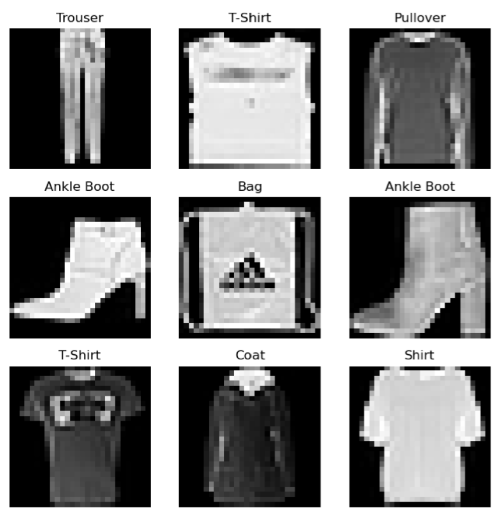
Now we’ll get familiar with the data we’ll be using, the Fashion MNIST dataset. This dataset contains 70,000 grayscale images of articles of clothing — 60,000 meant to be used for training and 10,000 meant for testing. The images are square and contain 28 × 28 = 784 pixels, where each pixel is represented by a value between 0 and 255. Each of these images is associated with a label, which is an integer between 0 and 9 that classifies the article of clothing. The following dictionary helps us understand the clothing categories corresponding to these integer labels:

https://github.com/bstollnitz/fashion-mnist-tf/blob/main/fashion-mnist-tf/local-keras/src/main.py

...
labels_map = {
    0: 'T-Shirt',
    1: 'Trouser',
    2: 'Pullover',
    3: 'Dress',
    4: 'Coat',
    5: 'Sandal',
    6: 'Shirt',
    7: 'Sneaker',
    8: 'Bag',
    9: 'Ankle Boot',
}
...

Here’s a random sampling of 9 images from the dataset, along with their labels:

Sample of the Fashion MNIST dataset.

Keras Dataset and data transformation

Keras provides us with an easy way to get some of the most popular datasets through tf.keras.datasets, and Fashion MNIST is no exception. We can simply call the load_data() method of the Fashion MNIST dataset, and we get back two tuples of NumPy arrays containing the training and test data and labels.

https://github.com/bstollnitz/fashion-mnist-tf/blob/main/fashion-mnist-tf/local-keras/src/main.py

...
def _get_data(batch_size: int) -> Tuple[tf.data.Dataset, tf.data.Dataset]:
    """Downloads Fashion MNIST data, and returns two Dataset objects
    wrapping test and training data."""
    (training_images, training_labels), (
        test_images, test_labels) = tf.keras.datasets.fashion_mnist.load_data()

    train_dataset = tf.data.Dataset.from_tensor_slices(
        (training_images, training_labels))
    test_dataset = tf.data.Dataset.from_tensor_slices(
        (test_images, test_labels))

    train_dataset = train_dataset.map(lambda image, label:
                                      (float(image) / 255.0, label))
    test_dataset = test_dataset.map(lambda image, label:
                                    (float(image) / 255.0, label))

    train_dataset = train_dataset.batch(batch_size).shuffle(500)
    test_dataset = test_dataset.batch(batch_size).shuffle(500)

    return (train_dataset, test_dataset)
...

For such a small dataset, we could just use the NumPy arrays given to us by Keras to train the neural network. However, if we had a large dataset, we would need to wrap it in a tf.data.Dataset instance, which handles large data better by making it easy to keep just a portion of it in memory. I’ve decided to wrap our data in a Dataset in this blog post, so you’re prepared to work with large data in the future.

As I mentioned, each image consists of 784 pixels, and each pixel is of type unsigned int and contains a value between 0 and 255. In machine learning, we generally want the pixel values of our training data to be floating-point numbers between 0 and 1. Therefore, we convert each pixel into a floating-point number between 0 and 1, by dividing its value by 255.0.

We then tell the Dataset to give us (shuffled) batches of data of the size passed in as a parameter to this function. This means that when we iterate over the Dataset, we receive not one, but a batch of batch_size items instead. Why do we want batches? We’ll come back to that in the section on training. But first we need to learn about the neural network architecture we’ll use for this sample.

Neural network architecture

Our goal is to classify an input image into one of the 10 classes of clothing, so we will define our neural network to take as input a matrix of shape (28, 28) and output a vector of size 10, where the index of the largest value in the output corresponds to the integer label for the class of clothing in the image. For example, if we use an image of an ankle boot as input, we might get an output vector like this:

In this particular example, the largest value appears at index 9 (counting from zero) — and as we showed in the previous section, index 9 corresponds to the “Ankle Boot” category. So this indicates that our neural network correctly classified the image of an ankle boot.

Here’s a visualization of the structure of the neural network we chose for this scenario:

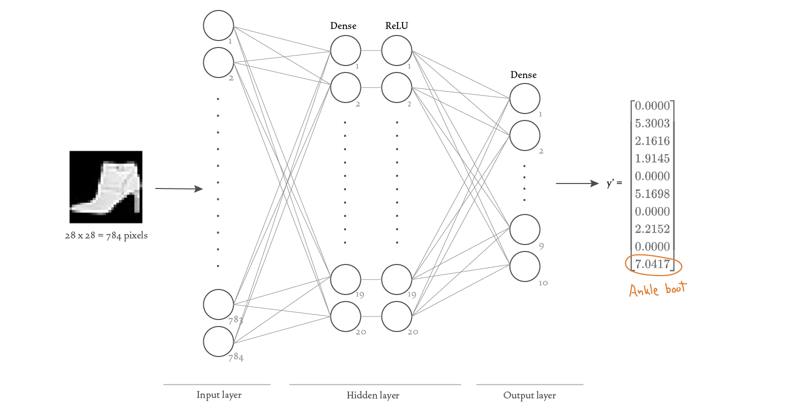
Diagram of Fashion MNIST classification neural network.

Because each image has 28 × 28 = 784 pixels, we need 784 nodes in the input layer (one for each pixel value). We decided to add one hidden layer with 20 nodes and a ReLU (rectified linear unit) activation function. We want the output of our network to be a vector of size 10, therefore our output layer needs to have 10 nodes.

Here’s the Keras code that defines this neural network:

https://github.com/bstollnitz/fashion-mnist-tf/blob/main/fashion-mnist-tf/local-keras/src/neural_network.py

import tensorflow as tf

class NeuralNetwork(tf.keras.Model):
    """Neural network that classifies Fashion MNIST-style images."""

    def __init__(self):
        super().__init__()
        self.sequence = tf.keras.Sequential([
            tf.keras.layers.Flatten(input_shape=(28, 28)),
            tf.keras.layers.Dense(20, activation='relu'),
            tf.keras.layers.Dense(10)
        ])

    def call(self, x: tf.Tensor) -> tf.Tensor:
        y_prime = self.sequence(x)
        return y_prime

The Flatten layer turns our input matrix of shape (28, 28) into a vector of size 728. The Dense layers are also known as “fully connected” or “linear” layers because they connect all nodes from the previous layer with each of their own nodes using a linear function. The ReLU activation functions take the output of the Dense layer and pass it through a “Rectified Linear Unit” function, which adds non-linearity to the computation.

It’s important to have non-linear activation functions (like the ReLU function) between linear layers, because otherwise a sequence of linear layers would be mathematically equivalent to just one layer. These activation functions give our network more expressive power, allowing it to approximate non-linear relationships between data.

The Sequential class combines all the other layers. Lastly, we define the call method, which supplies a tensor x as input to the sequence of layers and produces the y_prime vector as a result.

Training the network

Let’s start by defining a couple of constants that we’ll use in the training and prediction code.

https://github.com/bstollnitz/fashion-mnist-tf/blob/main/fashion-mnist-tf/local-keras/src/main.py

MODEL_DIRPATH = 'fashion-mnist-tf/local-keras/model/weights'
IMAGE_FILEPATH = 'fashion-mnist-tf/local-keras/src/predict-image.png'

Now that we understand how to get the data and model, we’re ready to train the neural network. In order to understand what happens during training, we need to add a little more detail to our neural network visualization:

Basic neural network with details.

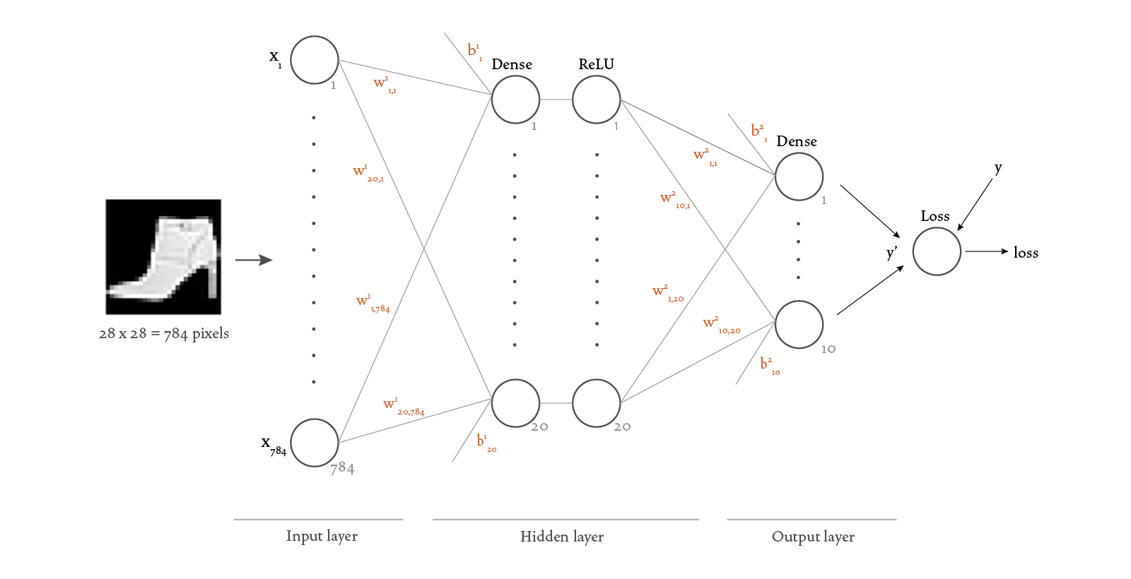
There’s a lot of new information in this diagram, so I’ll expand on each of the new concepts here.

Notice that we’ve added weights to the connections between layers, and bias as input to Dense layers — and are the neural network’s parameters. Our goal when training our network (also known as fitting) is to find the parameters and that minimize the differences between the actual and predicted labels for our data.

Notice also that we added a Loss function to the diagram. This function takes in the outputs of the model (the predicted labels) and the actual labels , measures their differences, and combines those into a single output, which we call the loss. The loss gives us a single number that quantifies how similar our predictions are to the actual labels: a high loss indicates that they’re different, and a low loss indicates that our predictions are accurate. The loss function most frequently used in classification is cross-entropy loss, and Keras provides several varieties of this loss. Because our dataset includes a single integer label for each example, we use the SparseCategoricalCrossentropy loss function.

Now let’s look at what happens in the Dense layers. Dense layers add a linear operation involving the input data and parameters and . For example, the top node of the first Dense layer performs the following calculation:

If we specify a ReLU activation function, the output of the linear operation is then passed as input to a ReLU function:

Mathematically speaking, we can now think of our neural network as a function that takes as input the data , expected labels , and parameters and , then performs a sequence of operations on that data, and returns a loss.

Our goal is to find the parameters and that lead to the lowest possible loss. (We can’t change our data or the corresponding labels — they’re fixed — but we can adjust and .) It turns out that problems of this kind fall in the well-studied mathematical area of optimization. The simplest minimization algorithm is gradient descent, and in this sample we use a variation known as Stochastic Gradient Descent or SGD. The training process is roughly as follows: First, the parameters and are initialized to random values. We then make predictions using those values, and evaluate the loss function to measure the quality of the predictions. And last, we use the optimizer to adjust the values of and such that the loss will be a bit lower next time. We repeat this process until we’ve found parameters that give us a very small loss value and good predictions.

We’re now ready to “compile” the model — this is where we tell it that we want to use the SGD optimizer and the SparseCategoricalCrossentropy loss function. We also tell the model that we want it to report on the accuracy during training.

https://github.com/bstollnitz/fashion-mnist-tf/blob/main/fashion-mnist-tf/local-keras/src/main.py

...
def training_phase():
    """Trains the model for a number of epochs, and saves it."""
    learning_rate = 0.1
    batch_size = 64
    epochs = 5

    (train_dataset, test_dataset) = _get_data(batch_size)

    model = NeuralNetwork()

    loss_fn = tf.keras.losses.SparseCategoricalCrossentropy(from_logits=True)
    optimizer = tf.keras.optimizers.SGD(learning_rate)
    metrics = ['accuracy']
    model.compile(optimizer, loss_fn, metrics)

    print('\n***Training***')
    model.fit(train_dataset, epochs=epochs)

    print('\n***Evaluating***')
    (test_loss, test_accuracy) = model.evaluate(test_dataset)
    print(f'Test loss: {test_loss:>8f}, ' +
          f'test accuracy: {test_accuracy * 100:>0.1f}%')

    model.save(MODEL_DIRPATH)
...

A few details from the code above deserve a quick explanation.

Notice that we pass from_logits=True to the loss function. This is because the categorical cross-entropy function requires a probability distribution as input, meaning that the numbers should be between zero and one, and they should add up to one. Our network produces a vector of numbers that have no upper or lower bound (called “logits”), so we need to normalize them to get a probability distribution. This is typically done using the softmax function, and specifying from_logits=True automatically calculates the softmax before computing the loss.

Notice also that we pass a learning_rate to the SGD optimizer. The learning rate is a parameter needed in the gradient descent algorithm. We could have left it at the default, which is 0.01. But it’s important to know how to specify it because different learning rates can lead to very different prediction accuracies.

Finally, notice that we specified a batch_size, which we used in the construction of the Dataset, as we saw earlier. This is important during training, because it tells the model that we want to train on 64 images at a time. You might be wondering why 64? Why not train on a single image at a time? Or all 60,000 images at once? Doing a complete training step for each individual image would be inefficient because we would have to perform all the calculations 60,000 times in order to account for every input image. If we included all the input images in , we’d need a lot of memory, and we’d spend a lot of time computing each training step. So we settle for a size in between, called the “mini-batch” size.

Now that we’ve configured our model with the parameters we need for training, we can call fit to train the model. We specify the number of epochs as 5, which means that we want to iterate over the complete set of 60,000 training images five times while training the neural network.

Running the previous code produces the output below, showing that the accuracy tends to increase and the loss tends to decrease as we run more epochs.

***Training***
Epoch 1/5
938/938 [==============================] - 7s 5ms/step - loss: 0.6382 - accuracy: 0.7764
Epoch 2/5
938/938 [==============================] - 6s 5ms/step - loss: 0.4709 - accuracy: 0.8327
Epoch 3/5
938/938 [==============================] - 6s 5ms/step - loss: 0.4327 - accuracy: 0.8463
Epoch 4/5
938/938 [==============================] - 5s 5ms/step - loss: 0.4109 - accuracy: 0.8530
Epoch 5/5
938/938 [==============================] - 5s 5ms/step - loss: 0.3962 - accuracy: 0.8593

Training has found values for the parameters and such that, when we provide an image as input, we’ll get a reasonable prediction as output.

You may have noticed that we have a call to model.evaluate(...) in the code we showed above. Let’s take a look at that next.

Testing the network

After we’ve trained the network and have found parameters and that we believe will effectively predict the class of an image, it’s time to test or evaluate our network. Remember that earlier we set aside 10,000 images for testing, and created a Dataset using that data. We’ll use it now. You’ve already seen this code as part of the training_phase() function, but we’ll show it here again:

https://github.com/bstollnitz/fashion-mnist-tf/blob/main/fashion-mnist-tf/local-keras/src/main.py

    ...
    (test_loss, test_accuracy) = model.evaluate(test_dataset)
    ....

Running the previous code produces output similar to this:

***Evaluating***
157/157 [==============================] - 1s 4ms/step - loss: 0.4883 - accuracy: 0.8197

We’ve achieved pretty good test accuracy, considering that we used such a simple network and only five epochs of training.

Making predictions

We can now use the trained model for inference — in other words, to predict the classification of images.

Making a prediction is easy — we simply call the model’s predict method and pass one or more images. In our scenario, we’ll predict the label for the following image:

Image of an ankle boot.

In the code below, we load the image, call predict to get its class index, and map that index to the class name.

https://github.com/bstollnitz/fashion-mnist-tf/blob/main/fashion-mnist-tf/local-keras/src/main.py

...
def inference_phase():
    """Makes a prediction for a local image."""
    print('\n***Predicting***')

    model = tf.keras.models.load_model(MODEL_DIRPATH)

    with Image.open(IMAGE_FILEPATH) as image:
        x = np.asarray(image).reshape((-1, 28, 28)) / 255.0

    predicted_index = np.argmax(model.predict(x))
    predicted_name = labels_map[predicted_index]

    print(f'Predicted class: {predicted_name}')
...

***Predicting***
Predicted class: Ankle Boot

Saving and loading

For the sake of simplicity, the code sample for this post includes the training, testing, and prediction phases in one program. In practice, though, training and testing are performed together, while prediction is often done in a separate program, executed at a different time or on a different machine. To help with this scenario, Keras offers a variety of ways to save and load a trained neural network model.

In this project, at the end of the fitting and evaluation phases, we save the model by executing the following code:

https://github.com/bstollnitz/fashion-mnist-tf/blob/main/fashion-mnist-tf/local-keras/src/main.py

    ...
    model.save(MODEL_DIRPATH)
    ...

Then, once we’re ready to do inference, we load it back into memory:

https://github.com/bstollnitz/fashion-mnist-tf/blob/main/fashion-mnist-tf/local-keras/src/main.py

    ...
    model = tf.keras.models.load_model(MODEL_DIRPATH)
    ...

For more information and alternative techniques, see the Keras tutorial on saving and loading models.

Conclusion

Thank you so much for sticking with this blog post until the end. You learned a lot, and now you have the basic tools to make predictions on your own data using Keras. You learned how to prepare your data, how to define your neural network, how to train and test it, and finally how to make a prediction using your trained network.

The complete code for this post can be found on GitHub.

Thank you to Laurence Moroney from Google and Dmitry Soshnikov from Microsoft for reviewing the content in this post.