Using PySINDy to discover equations from experimental data
Created:
Topic: Scientific ML techniques
Introduction
In my post about the 2016 SINDy paper by Brunton et al., I showed how to implement the ideas in that paper from scratch, and discovered the nonlinear three-dimensional Lorenz system based solely on data samples. However, the data samples were generated using the Lorenz system itself. This was a good approach to give us confidence that the method works, but in a real-world application we don’t know what the system is during data generation — that’s the whole point of SINDy, to discover the system!
In this post, we’ll collect our data experimentally, and then use the PySINDy package to discover the system that describes it. PySINDy provides us with an API that implements the ideas in the original SINDy paper, along with some improvements from subsequent papers. This is super convenient — in a real-world project there’s no reason to reinvent the wheel by providing our own implementation!
The Python code for this project can be found on github. All the files mentioned in this blog post are under the sindy/oscillator-pysindy directory.
I divided the code into the following three main sections, each in its own file:
1_process_data.py— Gathers the data. 2_fit.py— Uses PySINDy to find sparse equations that best represent the data.3_predict.py— Predicts a trajectory, given an initial condition and the equations discovered by PySINDy.
Let’s start by discussing how we gather the data.
Gathering our data
In this project, we want to discover a system of ordinary differential equations that describes the trajectory of the paint can in this video:
Our first task is to collect data points for our experiment — in this case our data points represent the position of the paint can over time. We could have taken many different approaches in the representation of this data. In this project our data
https://github.com/bstollnitz/sindy/tree/main/sindy/oscillator-pysindy/src/utils_video.py
import logging
from typing import Tuple

import cv2
import numpy as np
from tqdm import tqdm

def track_object(input_file_path: str, bbox: Tuple[int],
                 output_file_path: str) -> np.ndarray:
    """
    Tracks an object in a video defined by the bounding box passed
    as a parameter. Saves an output video showing the bounding box found.
    Returns an ndarray of shape (frames, 2) containing the
    (x, y) center of the bounding box in each frame.
    """
    logging.info("Tracking object.")

    # Open video.
    capture = cv2.VideoCapture(input_file_path)
    if not capture.isOpened():
        raise Exception(f"Could not open video: {input_file_path}.")

    # Define tracker.
    tracker = cv2.TrackerCSRT_create()

    # Get the codec for an AVI file.
    fourcc = cv2.VideoWriter_fourcc(*"XVID")

    # Read each frame of the video, gather centers of all bounding boxes, and
    # save video showing those bounding boxes.
    color = (0, 0, 255)
    writer = None
    centers = []
    frame_count = int(capture.get(cv2.CAP_PROP_FRAME_COUNT))
    for i in tqdm(range(frame_count)):
        (ok, frame) = capture.read()
        if not ok:
            raise Exception(f"Cannot read video frame {i}.")

        if i == 0:
            # Uncomment this to select a bounding box interactively.
            # bbox = cv2.selectROI("Frame",
            #                      frame,
            #                      fromCenter=False,
            #                      showCrosshair=True)
            tracker.init(frame, bbox)
            writer = cv2.VideoWriter(output_file_path,
                                     fourcc,
                                     fps=30.0,
                                     frameSize=(frame.shape[1], frame.shape[0]))
        else:
            (ok, bbox) = tracker.update(frame)
            if not ok:
                raise Exception(f"Could not track object in frame {i}.")
        center = (bbox[0] + bbox[2] / 2, bbox[1] + bbox[3] / 2)
        centers.append(center)

        # Color the bounding box and center of an output video frame.
        x = int(center[0])
        y = int(center[1])
        fill_rectangle(frame, (x - 2, y, 2, 5, 5), color)
        outline_rectangle(frame, bbox, color)
        writer.write(frame)

    capture.release()
    writer.release()

    return np.asarray(centers)
In the code above, the first parameter passed to the function is the path to the input video file, which we’ll open using OpenCV’s VideoCapture(...) function. We also receive the coordinates of the bounding box of the paint can in the first frame of the input video, in format (left, top, width, height). Then for each frame of the input video, we read it, get the bounding box for the paint can in that frame, calculate its center, and append the center to the centers list. In addition, we also receive as parameter a path to where we’ll save an output video file. This file contains the input video with the tracker findings overlayed on top of it: a red outline representing the bounding box around the paint can, and a red dot in its center. The (x, y) coordinates of the center dots over time make up our data matrix
Let’s take a look at the video with the overlays:
Then, in the main function of the 1_processs_data.py file, we call the function that collects the data
https://github.com/bstollnitz/sindy/tree/main/sindy/oscillator-pysindy/src/1_processs_data.py
from pathlib import Path
from utils_video import track_object
import numpy as np

def main() -> None:
    ...
    input_file_name = "damped_oscillator_900.mp4"
    input_file_path = str(Path(original_data_dir, input_file_name))
    bbox = (269, 433, 378, 464)
    Path(data_dir).mkdir(exist_ok=True)
    output_file_name = "damped_oscillator_900_tracked.avi"
    output_file_path = str(Path(data_dir, output_file_name))
    u = track_object(input_file_path, bbox, output_file_path)

    t = np.arange(stop=u.shape[0])
    ...
You may be wondering how you can figure out the bounding box of the paint can in the first frame. How did I come up with the coordinates (269, 433, 378, 464) in the code above? I found two ways that worked well for me:
- If you have access to Adobe Creative Cloud, you can open the video in Adobe Premiere Pro, export its first frame, open it in Adobe Photoshop, and get the coordinates for the top left corner, width and height.
- Otherwise, you can get the coordinates interactively through code. I left the code that provides this functionality in the project, commented out, in case you’d like to follow this approach in your project:
https://github.com/bstollnitz/sindy/tree/main/sindy/oscillator-pysindy/src/utils_video.py
        ...
        if i == 0:
            # Uncomment this to select a bounding box interactively.
            # bbox = cv2.selectROI("Frame",
            #                      frame,
            #                      fromCenter=False,
            #                      showCrosshair=True)
            tracker.init(frame, bbox)
            writer = cv2.VideoWriter(output_file_path,
                                     fourcc,
                                     fps=30.0,
                                     frameSize=(frame.shape[1], frame.shape[0]))
        ...
And that’s all there is to it. We have our data
Fitting using PySINDy
If you try to ask PySINDy for a model by simply giving it all the data collected in the previous section, you won’t get great results. Machine learning is a powerful tool, but you still have to think and use good judgement. We may not know the exact equations of the movement, but we can use basic knowledge of ordinary differential equations to make some guesses that will help guide PySINDy in the right direction.
Let’s first consider the vertical movement of the paint can. This movement resembles that of the well-studied damped harmonic oscillator, which can be represented by the following second-order linear equation:
So, we can make an informed guess that our vertical coordinate
Therefore, in order to make use of our assumption, we need to first turn the second-order damped harmonic oscillator equation into a system of two first-order equations. We can do that with the aid of two new variables,
The equation can then be re-written as the following system:
This is great information to have, because we now know that the vertical movement most likely needs two coordinates to be represented as a system of first-order equations: one of them being the
Now let’s consider the horizontal movement of the paint can. This time the movement resembles a pendulum, and we also have a well-studied ordinary differential equation that represents that trajectory. However, the movement is so slight that the damped harmonic oscillator equation is probably a good enough approximation for our purposes. It’s also much simpler than the pendulum equation, which would require a change of variables (great topic for a future post). Therefore, we’ll use the exact same technique to help PySINDy understand the horizontal movement: we’ll assume that it needs two coordinates, one of them being the
You could try giving PySINDy data for these four coordinates, but I found that I get better results if I treat the horizontal and vertical movements as independent. As you can see in the code below, I create two independent PySINDy models, one for the horizontal movement, and another for the vertical movement:
https://github.com/bstollnitz/sindy/tree/main/sindy/oscillator-pysindy/src/2_fit.py
import logging
from typing import Tuple

import numpy as np
import pysindy as ps
from pysindy.differentiation import FiniteDifference
from pysindy.optimizers import STLSQ

from common import MAX_ITERATIONS, THRESHOLD

def fit(u: np.ndarray,
        t: np.ndarray) -> Tuple[ps.SINDy, ps.SINDy, np.ndarray, np.ndarray]:
    """Uses PySINDy to find the equation that best fits the data u.
    """
    optimizer = STLSQ(threshold=THRESHOLD, max_iter=MAX_ITERATIONS)

    differentiation_method = FiniteDifference()
    # pylint: disable=protected-access
    udot = differentiation_method._differentiate(u, t)

    # Get a model for the movement in x.
    logging.info("Model for x")
    x = u[:, 0:1]
    xdot = udot[:, 0:1]
    datax = np.hstack((x, xdot))
    modelx = ps.SINDy(optimizer=optimizer,
                      differentiation_method=differentiation_method,
                      feature_names=["x", "xdot"],
                      discrete_time=False)
    modelx.fit(datax, t=t, ensemble=True)
    modelx.print()
    logging.info("coefficients: %s", modelx.coefficients().T)

    # Get a model for the movement in y.
    logging.info("Model for y")
    y = u[:, 1:2]
    ydot = udot[:, 1:2]
    datay = np.hstack((y, ydot))
    modely = ps.SINDy(optimizer=optimizer,
                      differentiation_method=differentiation_method,
                      feature_names=["y", "ydot"],
                      discrete_time=False)
    modely.fit(datay, t=t, ensemble=True)
    modely.print()
    logging.info("coefficients: %s", modely.coefficients().T)

    return (modelx, modely, xdot, ydot)

def main() -> None:
    ...
    (modelx, modely, xdot, ydot) = fit(u, t)
    ...
Notice that I give each model two coordinates, one with spatial measurements gathered by the tracker and another with its derivatives (calculated using the Finite Differences method). Notice also that I choose the Sequential Thresholded Least-Squares (STLSQ) method to find a sparse set of candidate functions. I explain this algorithm in detail in my previous post.
If I set THRESHOLD to 0.001 and MAX_ITERATIONS to 100, PySINDy discovers the following coefficients and systems:
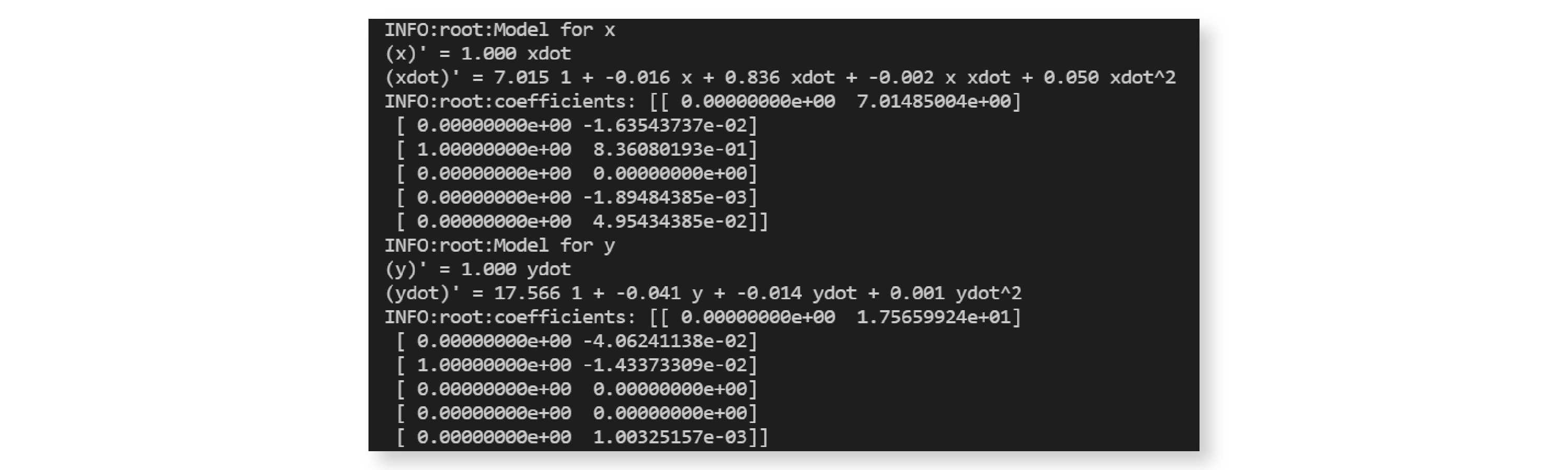
We discovered systems of ordinary differential equations for both types of movement! But can they predict the trajectory of a bouncing paint can? Let’s take a look in the next section.
Prediction of trajectory
In this section, we’ll use the two models to predict trajectories for the horizontal and vertical movements of the paint can. In order to get a trajectory, we need to specify initial conditions for our coordinates simulate(...) function from the model to get the predicted trajectory:
https://github.com/bstollnitz/sindy/tree/main/sindy/oscillator-pysindy/src/3_predict.py
def main() -> None:
    ...
    u0x = np.array([u[0, 0], xdot[0, 0]])
    u_approximation_x = modelx.simulate(u0x, t)

    u0y = np.array([u[0, 1], ydot[0, 0]])
    u_approximation_y = modely.simulate(u0y, t)
    ...
Let’s visualize our predicted trajectory for
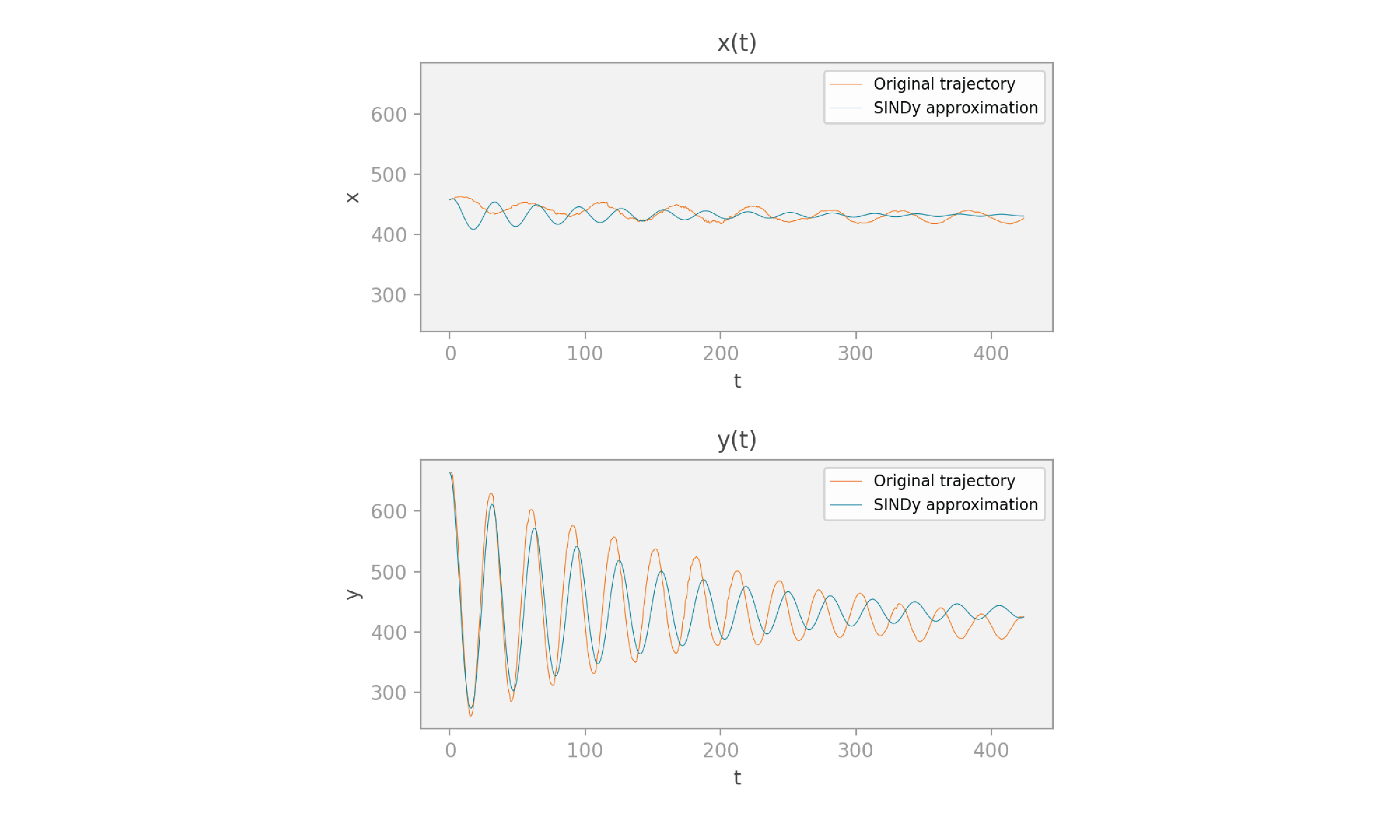
Not too bad. Especially if we take into account that our data
Conclusion
In this blog post, you saw how to predict the trajectory of an object being tracked in a video. First, you saw how to use OpenCV to collect the center coordinates of the object over time. Then, you saw how to use the data and the PySINDy package to discover sparse systems of two first-order ordinary differential equations that describe the horizontal and vertical movements that we observed. And finally, you saw how to use the systems to predict trajectories for the object, and compared those with the original trajectories.
The complete Python code for this project can be found on github.
Hopefully this gives you some ideas on how you can use PySINDy with your own experimental data. Thank you for reading, and best of luck for your SINDy applications!