Introduction

Suppose you’ve collected data from a physical system, and you need to make predictions based on that data. You could try training a neural network on your data, then use the neural network to make predictions — this might work for dynamics similar to the observed ones. However, it won’t help you understand the underlying physics of the system, and it won’t enable you to generalize to other systems governed by the same physical principles but with different characteristics. For example, a neural network trained on data from a swinging pendulum might always predict that a pendulum swings back and forth. However, if we learned the underlying physical equation, we could predict that when the angular velocity is large enough, it will transition to a motion where it rotates continuously in one direction. This ability to extrapolate has the potential to advance the physical sciences through new discoveries.

In this blog post, I’ll discuss one popular method for discovering governing equations for nonlinear dynamical systems: SINDy (Sparse Identification of Nonlinear Dynamics). The code and text in this post are based on the 2016 paper “Discovering governing equations from data by sparse identification of nonlinear dynamical systems” by Brunton, Proctor, and Kutz, and its accompanying Matlab code.

This is a useful technique if you’ve gathered data that evolves over time, and want to find a system of ordinary differential equations (ODEs) that describes and predicts this evolution. Scenarios that fall in this category are common in the physical sciences, such as biology, climate science, and neuroscience. In this post, we’ll use the nonlinear three-dimensional Lorenz system of equations as a basis for our experiments. But the main ideas you’ll learn here can be applied to any observed data that you suspect can be represented as a system of ODEs.

My Python code can be found on github. I encourage you to follow along on github as you read this article — the files I will mention are all under the sindy/lorenz-custom and sindy/lorenz-pysindy directories.

The main idea of the paper

SINDy aims to learn nonlinear dynamical systems from data. Assume we observe a sequence of -dimensional data points that are samples of some unknown trajectory . Our goal is to find a nonlinear dynamical system that governs the behavior of , of the following form:

We suppose that is a weighted sum of nonlinear terms, and our goal is to discover which terms make up , and their corresponding weights. The key idea from the paper is that is most likely a sparse function (with few terms), and we can find its terms by enforcing sparsity while performing linear regression. It’s a simple and powerful idea, which we’ll explore in detail in the rest of this post.

Note that the original SINDy paper and this post focus on systems of ordinary differential equations (meaning that is only a function of time), but subsequent work demonstrates that this technique also works for partial differential equations (where may be a function of time and space, or other variables). Maybe that’s a topic for a future post.

I’ll start by reminding you of the basics of linear regression. This is a foundational concept, and you can skip the next section if you already understand it well.

Linear regression

We’ll take a brief look at linear regression in this section.

The goal of linear regression is to model the relationship between two variables, an -dimensional independent variable and a scalar-valued dependent variable, using a linear equation to relate the two. In machine learning, typically, the -dimensional independent variable consists of the data point’s features, and the scalar-valued dependent variable holds the corresponding target value.

Let’s look at the equation that describes the linear relationship that we would like to establish between these two variables:

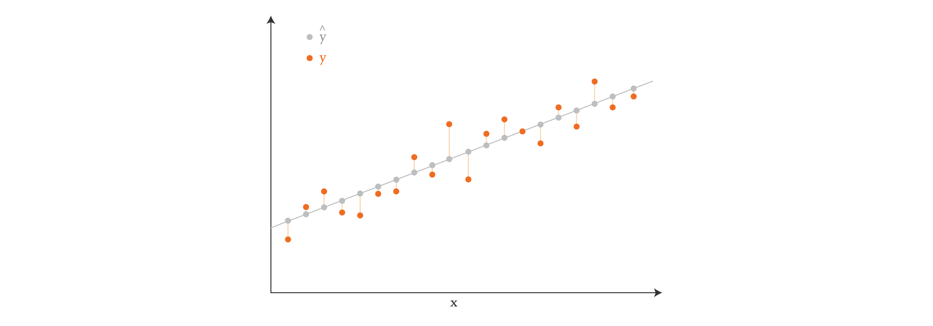
We’ll assume that we have data points, each with features, forming the matrix . We also have a vector of size containing a target value associated with each data point. In general, it’s impossible to satisfy the equation above exactly. Instead, our goal is to find coefficients for the weight vector and bias such that the right-hand-side of the equation above (which we’ll call ) comes as close as possible to the left-hand-side . Here, the weight vector is of size , and the bias vector is of size , where the constant bias is repeated times.

Visually, if our data points have just one feature (so has one column), we can think of linear regression as finding a line in 2D that comes closest to passing through all the points , where is a row of , and is the corresponding target value. In the diagram below, the orange dots show the target values , and the gray dots show the predictions .

Image showing the linear regression line going through data points

If our data points were two-dimensional, then we would be finding a plane instead of a line. And if they were -dimensional, we would be finding a hyperplane.

In the context of machine learning, it’s common to write the relationship between and by incorporating into the rest of the equation, which avoids the repetition of the constant bias:

In this equation, now has size , where the entries in the first column are all . The unknown vector is now , of size , because it contains the value of the constant bias in the first row followed by the values of . The vector has the same size as before, , as expected.

In the equation above, the target values and the features are known, so our goal is to find the vector that makes the right-hand-side of the equation best approximate the left-hand-side. Problems of this kind are often solved directly using least-squares techniques (like the normal equation), which aim to minimize the square of the distance between the predicted values and target values — in other words, they minimize the sum of the lengths of the vertical lines in the diagram above. Problems of this kind can also be solved using iterative optimization methods, such as gradient descent, which grant us more freedom in our approach.

Often our goal is not just to get the best — we want the best that is also sparse. Sparsity is a desirable feature in general, and we’ll see later why sparsity is super important in the SINDy scenario in particular. It turns out that there are also several algorithms that help us solve the equation above with sparsity — for example, LASSO (Least Absolute Shrinkage and Selection Operator) is a popular method.

Back to main idea of the paper

So, how do linear regression and sparsity relate to the SINDy paper? Remember the ordinary differential equation that we’re trying to find:

We have samples of at several times, and nothing else. But if we have , we can easily calculate using a numerical method (such as finite differences, or total variation with regularization, as suggested by the authors in the paper). Our goal then is to find the function that best represents the behavior of the derivative of over time. One way to represent is by thinking of it as a linear combination of a set of candidate functions. These candidate functions can be polynomial functions, trigonometric functions, or anything else that might be a reasonable guess for the behavior of the derivatives.

For example, if someone else gives us data that was generated by the Lorenz system without telling us how it was generated, we would be successful in discovering the equations as long as we include low-degree polynomials in our set of candidate functions. That’s because the Lorenz system looks like this:

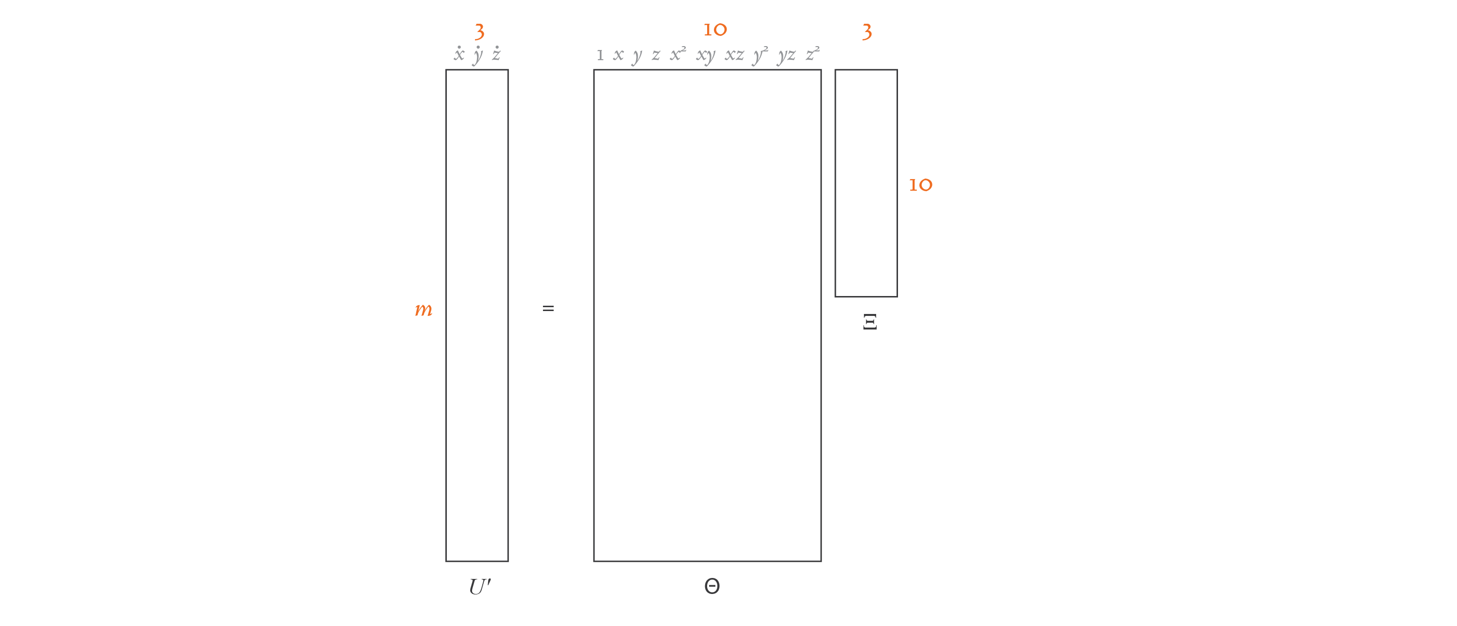
So, in this case, as long as we include , , , and in our set of candidate functions, we should be able to reconstruct the equations from the data.

In the general scenario, we can express the derivatives as a linear combination of candidate functions, as follows:

In the equation above, contains the derivatives. For the Lorenz equation, let’s assume that we collected three-dimensional samples. Then holds the time derivatives at each of those samples, and is of size .

The matrix contains possible candidate functions, and so it’s of size . We can consider any candidate function we’d like for , so we can define this matrix ahead of time. In our Lorenz system scenario, we’ll use low-degree polynomials as our candidate functions: , , , , , , , , , and . So, in this case.

The matrix is of size , and contains the coefficients that multiply the candidate functions. These coefficients are unknown, and it’s our goal to discover them.

Here’s a diagram that demonstrates the structure of our equation for this simple example:

$Image showing the dimensions of the U' = \Theta(U) \Xi equation for the Lorenz system$

If you compare this equation with the linear regression one in the previous section, you’ll see that the overall structure is the same. The only difference is that and are now matrices of width , not column vectors. That’s because instead of a single linear regression problem, we have linear regression problems, one for each dimension. If you split the equation above into separate equations, each containing a column of and the corresponding column of , you’d have problems with the exact same structure I showed in the linear regression section. Here’s an illustration of this idea:

Image showing the Lorenz system diagram, split into three subproblems

and are known, so we need to solve for . We could do that using a direct least-squares method. However, physical equations are typically best represented by just a few terms, so we need to be sparse. We may consider dozens of different candidate functions in , but in the end, we want only a few to be present in our function . So, in essence, this problem boils down to solving linear regression problems with sparsity.

As I mentioned earlier, LASSO is a popular method for solving linear regression problems while optimizing for a sparse solution. However, the authors of the paper found LASSO to be algorithmically unstable and computationally expensive for very large data sets, so they designed an alternative: the “Sequential Thresholded Least-Squares” algorithm.

Fitting using Sequential Thresholded Least-Squares

In the next three sections, I will explain each of the three main Python files in the accompanying project:

sindy/lorenz-custom/src/1_generate_data.py — Generates sample data and calculates its derivatives .
sindy/lorenz-custom/src/2_fit.py — Discovers a sparse equation that represents our data well, using the Sequential Thresholded Least-Squares algorithm.
sindy/lorenz-custom/src/3_predict.py — Uses the discovered equation to predict a trajectory, given an initial condition.

I’ll begin with the second file, since that’s where the SINDy paper brings the most innovation. Here’s my Python implementation of the Sequential Thresholded Least-Squares algorithm:

https://github.com/bstollnitz/sindy/tree/main/sindy/lorenz-custom/src/2_fit.py

import numpy as np

def calculate_regression(theta: np.ndarray, uprime: np.ndarray,
                         threshold: float, max_iterations: int) -> np.ndarray:
    """Finds a xi matrix that fits theta * xi = uprime, using the sequential
    thresholded least-squares algorithm, which is a regression algorithm that
    promotes sparsity.

    The authors of the SINDy paper designed this algorithm as an alternative
    to LASSO, because they found LASSO to be algorithmically unstable, and
    computationally expensive for very large data sets.
    """
    # Solve theta * xi = uprime in the least-squares sense.
    xi = np.linalg.lstsq(theta, uprime, rcond=None)[0]
    n = xi.shape[1]

    # Add sparsity.
    for _ in range(max_iterations):
        small_indices = np.abs(xi) < threshold
        xi[small_indices] = 0
        for j in range(n):
            big_indices = np.logical_not(small_indices[:, j])
            xi[big_indices, j] = np.linalg.lstsq(theta[:, big_indices],
                                                 uprime[:, j],
                                                 rcond=None)[0]

    return xi

In the code above, the theta input parameter contains the matrix of candidate functions, and the uprime input parameter contains the matrix with derivatives — these are known ahead of time. The output of this function is the matrix, which is initially unknown. The threshold and max_iterations input parameters help us fine-tune the Sequential Threasholded Least-Squares algorithm, as we’ll see soon.

The first operation in this algorithm is to calculate a least-squares solution to the equation using a direct method, which is a great starting point:

https://github.com/bstollnitz/sindy/tree/main/sindy/lorenz-custom/src/2_fit.py

    xi = np.linalg.lstsq(theta, uprime, rcond=None)[0]

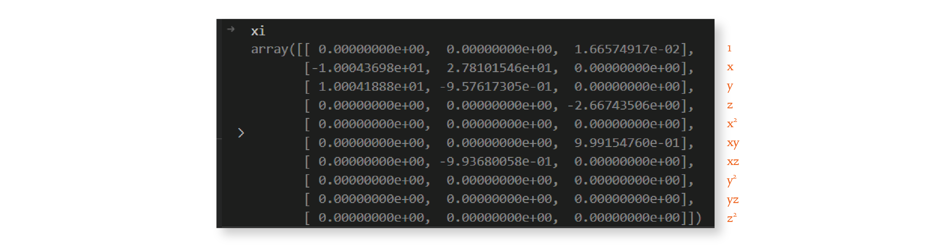
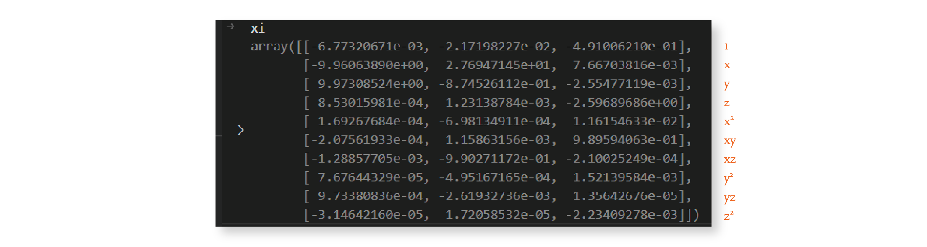
Below is one potential result for this operation. Remember that the matrix in our scenario has shape , because we’re considering 10 candidate functions and have 3 dimensions.

xi matrix, not sparse.

This matrix solves the equation, but as you can see, it’s not sparse. The role of the for loop that follows is to introduce sparsity to the matrix, while compromising as little as possible on the accuracy of the solution. The code first identifies all the matrix locations with coefficients smaller than the threshold passed as a parameter, and sets those coefficients to zero:

https://github.com/bstollnitz/sindy/tree/main/sindy/lorenz-custom/src/2_fit.py

    for _ in range(max_iterations):
        small_indices = np.abs(xi) < threshold
        xi[small_indices] = 0
        for j in range(n):
            big_indices = np.logical_not(small_indices[:, j])
            xi[big_indices, j] = np.linalg.lstsq(theta[:, big_indices],
                                                 uprime[:, j],
                                                 rcond=None)[0]

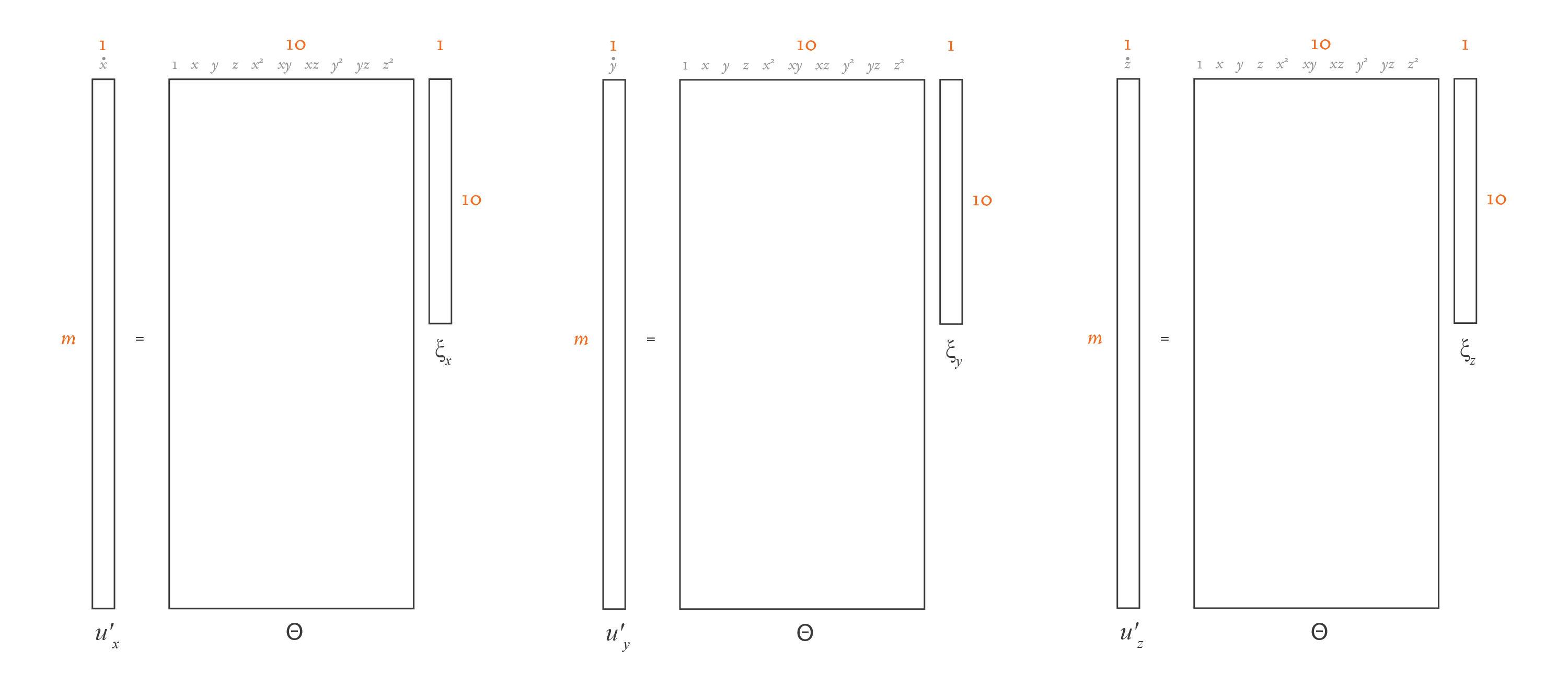
Then, it solves the least-squares problem considering only the remaining non-zero coefficients. However, because we may have a different number of non-zero coefficients in each column of , we need to break the problem into separate linear regression problems, one for each column of and corresponding column of . I showed this idea in the illustration at the end of the previous section.

Let’s look at what the matrix looks like after one iteration of the outer loop, with threshold value 0.025:

xi matrix, sparser.

The matrix is much sparser now. We repeat this procedure 9 more times because we set max_iterations to 10, and by the end, we have the following matrix:

xi matrix, final.

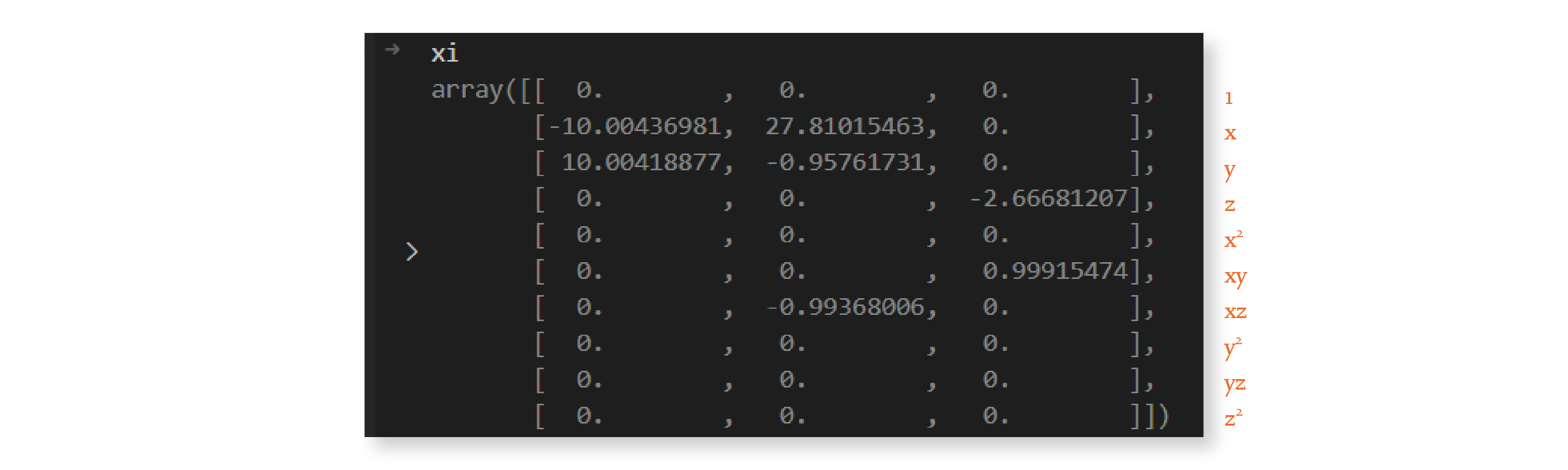
And we’re done — we discovered a sparse matrix! We can now use it to write down the equation of the system, rounded to two decimal places:

As you can see, the system discovered by this algorithm is very similar to the Lorenz system with parameters , , and . These are the parameter values I used in the generation of the input data, as we’ll see in the next section.

The small differences between the predicted and actual coefficients are due to noise in the calculation of the derivatives. We’ll also come back to this in the next section.

Let’s now take a look at the main function in this file. As you can see, it has two steps: it creates the library of candidate functions, and it uses the Sequential Thresholded Least-Squares algorithm to discover . The code that generates our data and its derivatives is in a different file, and will be the focus of the next section.

https://github.com/bstollnitz/sindy/tree/main/sindy/lorenz-custom/src/2_fit.py

from common import POLYNOMIAL_ORDER, USE_TRIG, THRESHOLD, MAX_ITERATIONS, create_library

def main() -> None:
    ...
    theta = create_library(u, POLYNOMIAL_ORDER, USE_TRIG)
    xi = calculate_regression(theta, uprime, THRESHOLD, MAX_ITERATIONS)
    ...

Let’s now look at the code that generates the matrix of candidate functions:

https://github.com/bstollnitz/sindy/tree/main/sindy/lorenz-custom/src/common.py

import numpy as np

def create_library(u: np.ndarray, polynomial_order: int,
                   use_trig: bool) -> np.ndarray:
    """Creates a matrix containing a library of candidate functions.

    For example, if our u depends on x, y, and z, and we specify
    polynomial_order=2 and use_trig=false, our terms would be:
    1, x, y, z, x^2, xy, xz, y^2, yz, z^2.
    """
    (m, n) = u.shape
    theta = np.ones((m, 1))

    # Polynomials of order 1.
    theta = np.hstack((theta, u))

    # Polynomials of order 2.
    if polynomial_order >= 2:
        for i in range(n):
            for j in range(i, n):
                theta = np.hstack((theta, u[:, i:i + 1] * u[:, j:j + 1]))

    # Polynomials of order 3.
    if polynomial_order >= 3:
        for i in range(n):
            for j in range(i, n):
                for k in range(j, n):
                    theta = np.hstack(
                        (theta, u[:, i:i + 1] * u[:, j:j + 1] * u[:, k:k + 1]))

    # Polynomials of order 4.
    if polynomial_order >= 4:
        for i in range(n):
            for j in range(i, n):
                for k in range(j, n):
                    for l in range(k, n):
                        theta = np.hstack(
                            (theta, u[:, i:i + 1] * u[:, j:j + 1] *
                             u[:, k:k + 1] * u[:, l:l + 1]))

    # Polynomials of order 5.
    if polynomial_order >= 5:
        for i in range(n):
            for j in range(i, n):
                for k in range(j, n):
                    for l in range(k, n):
                        for m in range(l, n):
                            theta = np.hstack(
                                (theta, u[:, i:i + 1] * u[:, j:j + 1] *
                                 u[:, k:k + 1] * u[:, l:l + 1] * u[:, m:m + 1]))

    if use_trig:
        for i in range(1, 11):
            theta = np.hstack((theta, np.sin(i * u), np.cos(i * u)))

    return theta

This function takes the data as a parameter, and uses it to calculate the numerical values for each of the candidate functions considered. In our scenario, we want to consider candidate polynomial functions up to order 2, so the polynomial_order parameter is set to 2. And we don’t want to consider trigonometric candidate functions, so the use_trig parameter is set to False.

Let’s now look at how we generate the data , and how we calculate its derivatives .

Generation of data and derivatives

In a real-world project, you would set up an experiment, and you would measure your data from observations. My next blog post will show one way to do this. But in this introductory project, to keep it simple, we’ll generate our data using the Lorenz equations.

Let’s see the code that generates :

https://github.com/bstollnitz/sindy/tree/main/sindy/lorenz-custom/src/1_generate_data.py

import numpy as np
from scipy.integrate import solve_ivp

from common import BETA, RHO, SIGMA


def lorenz(_: float, u: np.ndarray, sigma: float, rho: float,
           beta: float) -> np.ndarray:
    """Returns a list containing values of the three functions of the Lorenz system.

    The Lorenz equations have constant coefficients (that don't depend on t),
    but we still receive t as the first parameter because that's how the
    integrator works.
    """
    x = u[0]
    y = u[1]
    z = u[2]
    dx_dt = sigma * (y - x)
    dy_dt = x * (rho - z) - y
    dz_dt = x * y - beta * z

    return np.hstack((dx_dt, dy_dt, dz_dt))


def generate_u(t: np.ndarray) -> np.ndarray:
    """Simulates observed data u with the help of an integrator for the Lorenz
    equations.
    """
    u0 = np.array([-8, 8, 27])
    result = solve_ivp(fun=lorenz,
                       t_span=(t[0], t[-1]),
                       y0=u0,
                       t_eval=t,
                       args=(SIGMA, RHO, BETA))
    u = result.y.T
    return u

Here, we use SciPy’s solve_ivp function to get the Lorenz solution with initial value u0. If you’ve used Matlab before to work with differential equations, you likely used the ode45 function to solve them — solve_ivp is one way to do the same in Python. We need to tell the solve_ivp function the timesteps of our trajectory, which we store in variable t. In this case, the length of t determines the length of the trajectory returned by solve_ivp. We also need to specify the parameters of the Lorenz system, which we define elsewhere to be , , and .

We now have an array of three-dimensional values that represent a portion of a trajectory in the Lorenz system. But remember that we don’t need the actual data samples , we need their derivatives . There are many methods to calculate the derivatives of a function numerically. The authors of the paper suggest using total variation derivatives with regularization, because it’s more effective than simpler methods at keeping the noise to a minimum. I tried both total variation derivatives with regularization and the much simpler finite differences method, and for this simple problem, I get the same results. Therefore, I decided to use finite differences in my code, which I show below:

https://github.com/bstollnitz/sindy/tree/main/sindy/lorenz-custom/src/1_generate_data.py

from derivative import dxdt

def calculate_finite_difference_derivatives(u: np.ndarray,
                                            t: np.ndarray) -> np.ndarray:
    """Calculates the derivatives of u using finite differences.

    Finite difference derivatives are quick and simple to calculate. They
    may not do as well as total variation derivatives at denoising
    derivatives in general, but in our simple non-noisy scenario, they
    do just as well.
    """
    logging.info("Using finite difference derivatives.")
    uprime = dxdt(u.T, t, kind="finite_difference", k=1).T
    return uprime

I’m using the derivative Python package here, so I don’t need to provide my own implementation of the algorithm. You can use the same package to calculate total variation derivatives with regularization (which I show in the code for this project), among many other methods.

Using a numerical method to calculate derivatives will always introduce a bit of noise, which is why the equations we discovered aren’t exactly like the original ones, as you saw in the previous section. In this scenario, because we know the equations used to generate the data, we can generate exact derivatives by simply plugging our data into the differential equation. I also have code for this in the accompanying project, in case you’d like to give it a try. If you do try it, you’ll see that you’ll be able to recover the exact equations for the Lorenz system! However, keep in mind that in a real-world scenario we won’t have access to the equations (the whole point of using SINDy is to find them!), so we’ll always have some noise in our data and the resulting equations will never be 100% exact.

Let’s now look at the function that calls the code that generates and :

https://github.com/bstollnitz/sindy/tree/main/sindy/lorenz-custom/src/1_generate_data.py

def generate_data() -> Tuple[np.ndarray, np.ndarray]:
    """ Generates data u, and calculates its derivatives uprime.
    """
    t0 = 0.001
    dt = 0.001
    tmax = 100
    n = int(tmax / dt)
    t = np.linspace(start=t0, stop=tmax, num=n)

    # Step 1: Generate data u.
    u = generate_u(t)

    # Step 2: Calculate u' from u.
    uprime = calculate_finite_difference_derivatives(u, t)

    return (u, uprime)

As you can see, we create a list of timestamps t, which we then use in the two main steps of this file: the generation of the data , and the calculation of its derivatives . The main function then calls this function.

https://github.com/bstollnitz/sindy/tree/main/sindy/lorenz-custom/src/1_generate_data.py

def main() -> None:
    ...
    (u, uprime) = generate_data()
    ...

Making a prediction

In the last two sections, we explored the code in the following Python files:

sindy/lorenz-custom/src/1_generate_data.py — Generates our data from the Lorenz system, and calculates derivatives using the finite differences numerical method.
sindy/lorenz-custom/src/2_fit.py — Generates a matrix containing candidate functions for the equation we want to discover, and uses the Sequential Thresholded Least-Squares algorithm to discover that equation.

In this section, we’ll explore the code in the third and final file, sindy/lorenz-custom/src/3_predict.py, where we’ll make a prediction.

Let’s think about what it means to make a prediction in this scenario. In our “fit” code we discovered a system of ordinary differential equations based on our data. Therefore, if we’re given an initial condition, we should be able to integrate the differential equation we discovered and get a trajectory that predicts future values. We’ve already seen how to integrate an ordinal differential equation using the solve_ivp function, when we generated our data using the Lorenz equation. We’ll use the same technique here, except this time we want to integrate the differential equation we discovered:

We generated , calculated using finite differences, generated , and computed using Sequential Thresholded Least-Squares. We have all the pieces of the puzzle, and are now ready to understand the code that integrates the equation we discovered.

https://github.com/bstollnitz/sindy/tree/main/sindy/lorenz-custom/src/3_predict.py

import numpy as np
from scipy.integrate import solve_ivp

from common import POLYNOMIAL_ORDER, USE_TRIG, create_library

def lorenz_approximation(_: float, u: np.ndarray, xi: np.ndarray,
                         polynomial_order: int, use_trig: bool) -> np.ndarray:
    """For a given 1 x 3 u vector, this function calculates the corresponding
    1 x n row of the theta matrix, and multiples that theta row by the n x 3 xi.
    The result is the corresponding 1 x 3 du/dt vector.
    """
    theta = create_library(u.reshape((1, 3)), polynomial_order, use_trig)
    return theta @ xi


def compute_trajectory(u0: np.ndarray, xi: np.ndarray, polynomial_order: int,
                       use_trig: bool) -> np.ndarray:
    """Calculates the trajectory of the model discovered by SINDy.

    Given an initial value for u, we call the lorenz_approximation function
    to calculate the corresponding du/dt. Then, using a numerical method,
    solve_ivp uses that derivative to calculate the next value of u, using the
    xi matrix discovered by SINDy. This process repeats, until we have all
    values of the u trajectory.
    """
    t0 = 0.001
    dt = 0.001
    tmax = 100
    n = int(tmax / dt + 1)

    t = np.linspace(start=t0, stop=tmax, num=n)
    result = solve_ivp(fun=lorenz_approximation,
                       t_span=(t0, tmax),
                       y0=u0,
                       t_eval=t,
                       args=(xi, polynomial_order, use_trig))
    u = result.y.T

    return u

def main() -> None:
    ...
    u0 = np.array([-8, 8, 27])
    u_approximation = compute_trajectory(u0, xi, POLYNOMIAL_ORDER, USE_TRIG)
    ...

The compute_trajectory function should be familiar to you by now — it calculates a trajectory for the lorenz_approximation function, given an initial value and list of timestamps t. The lorenz_approximation function implements the equation we discovered. The result, u_approximation, is our prediction for the trajectory that starts at u0.

Let’s take a look at the original Lorenz trajectory, and the trajectory predicted by SINDy, side-by-side.

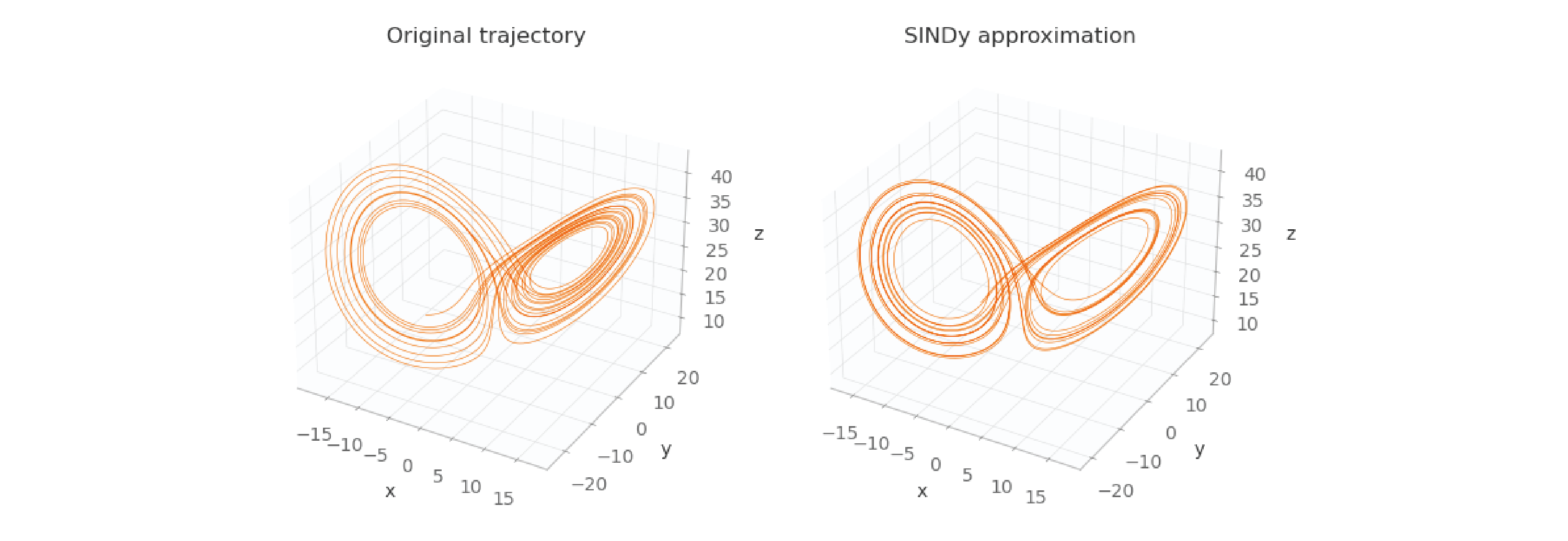
Original trajectory and SINDy approximation.

As you can see, the images aren’t exactly the same (because the equations discovered by SINDy aren’t exactly the same as the originals), but they’re very close. In the derivative calculation step, if instead of finite differences we had used exact derivatives, these two images would be exactly the same.

PySindy

Up until now, we explored the implementation of the basic ideas of SINDy, to help you understand its nuts and bolts. However, now that the PySINDy package is available, it’s much easier to just use that instead.

Let’s take a look at how the “fit” file changes if we use PySINDy. This code can be found on github under the sindy/lorenz-pysindy directory.

https://github.com/bstollnitz/sindy/tree/main/sindy/lorenz-pysindy/src/2_fit.py

import numpy as np
import pysindy as ps
from pysindy.differentiation import FiniteDifference
from pysindy.optimizers import STLSQ
from common import MAX_ITERATIONS, THRESHOLD

def fit(u: np.ndarray, t: np.ndarray) -> ps.SINDy:
    """Uses PySINDy to find the equation that best fits the data u.
    """
    optimizer = STLSQ(threshold=THRESHOLD, max_iter=MAX_ITERATIONS)
    differentiation_method = FiniteDifference()

    model = ps.SINDy(optimizer=optimizer,
                     differentiation_method=differentiation_method,
                     feature_names=["x", "y", "z"],
                     discrete_time=False)
    model.fit(u, t=t)
    model.print()
    logging.info("xi: %s", model.coefficients().T)

    return model

def main() -> None:
    ...
    model = fit(u, t)
    ...

This is much simpler than the previous project. Instead of implementing the Sequential Thresholded Least-Squares algorithm from scratch, we can simply call pysindy.optimizers.STLSQ(...). Also, we no longer need to create our own matrix — PySINDy takes care of that for us. We still need to specify a differentiation method, but now I can use the PySINDy API to do that, for convenience. I use FiniteDifferences here, but show how to use total variation derivatives with regularization in the project on github (I get the same results with both, just like before). The API is similar to other machine learning frameworks you might have used in the past: first we specify all the information the model needs, and then we call fit to train it. In this scenario, training means discovering the unknown coefficients for .

Then in the 3_predict.py file, instead of using the lower-level solve_ivp(...) method, we can now simply call model.simulate(...) to get our predicted trajectory.

https://github.com/bstollnitz/sindy/tree/main/sindy/lorenz-pysindy/src/3_predict.py


def compute_trajectory(u0: np.ndarray, model: ps.SINDy) -> np.ndarray:
    """Calculates the trajectory using the model discovered by SINDy.
    """
    t0 = 0.001
    dt = 0.001
    tmax = 100
    n = int(tmax / dt + 1)
    t_eval = np.linspace(start=t0, stop=tmax, num=n)

    u_approximation = model.simulate(u0, t_eval)

    return u_approximation

def main() -> None:
    ...
    u0 = np.array([-8, 8, 27])
    u_approximation = compute_trajectory(u0, model)
    ...

This code is also much simpler. Let’s now look at a visual representation of the original trajectory and the prediction made by PySINDy:

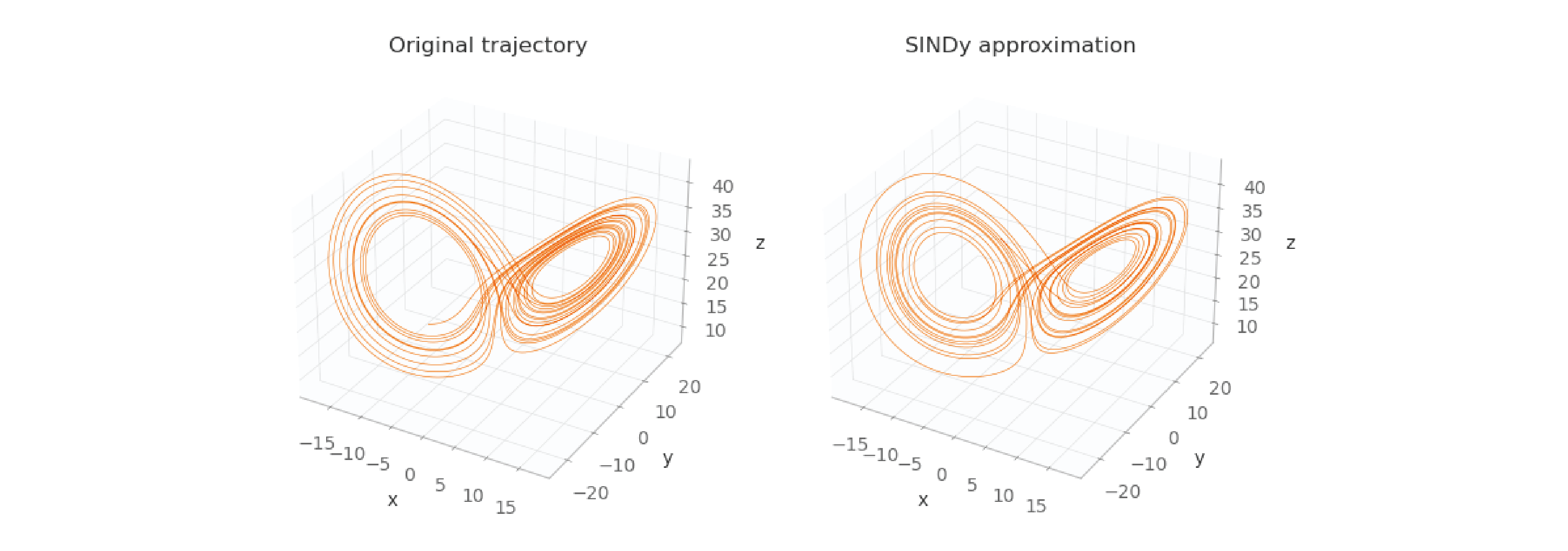
Original trajectory and PySINDy approximation.

The two trajectories are really close, maybe closer than the trajectory created using custom code. That’s likely because PySINDy implements not only the ideas of the original paper, but also improvements to those ideas made by many subsequent papers.

Conclusion

In this blog post, you learned about discovering non-linear systems of ordinary differential equations from data, using the ideas in the original SINDy paper. I first showed you how to implement the algorithms in the paper from scratch, and then I showed how to use the PySINDy API to accomplish the same task.

The Python code for this project can be found on github.

I hope that you learned something new, and that you’re inspired to use this technique with your own data. Thank you for reading!

Discovering equations from data using SINDy