The Transformer architecture of GPT models

Introduction

In 2017, authors from Google published a paper called Attention is All You Need in which they introduced the Transformer architecture. This new architecture achieved unparalleled success in language translation tasks, and the paper quickly became essential reading for anyone immersed in the area. Like many others, when I read the paper for the first time, I could see the value of its innovative ideas, but I didn’t realize just how disruptive the paper would be to other areas under the broader umbrella of AI. Within a few years, researchers adapted the Transformer architecture to many tasks other than language translation, including image classification, image generation, and protein folding problems. In particular, the Transformer architecture revolutionized text generation and paved the way for GPT models and the exponential growth we’re currently experiencing in AI.

Given how pervasive Transformer models are these days, both in the industry and academia, understanding the details of how they work is an important skill for every AI practitioner. This article will focus mostly on the architecture of GPT models, which are built using a subset of the original Transformer architecture, but it will also cover the original Transformer at the end. For the model code, I’ll start from the most clearly written implementation I have found for the original Transformer: The Annotated Transformer from Harvard University. I’ll keep the parts that are relevant to a GPT transformer, and remove the parts that aren’t. Along the way, I’ll avoid making any unnecessary changes to the code, so that you can easily compare the GPT-like version of the code with the original and understand the differences.

This article is intended for experienced data scientists and machine learning engineers. In particular, I assume that you’re well-versed in tensor algebra, that you’ve implemented neural networks from scratch, and that you’re comfortable with Python. In addition, even though I’ve done my best to make this article stand on its own, you’ll have an easier time understanding it if you’ve read my previous article on How GPT models work.

The code in this post can be found in the associated project on GitHub.

How to invoke our GPT Transformer

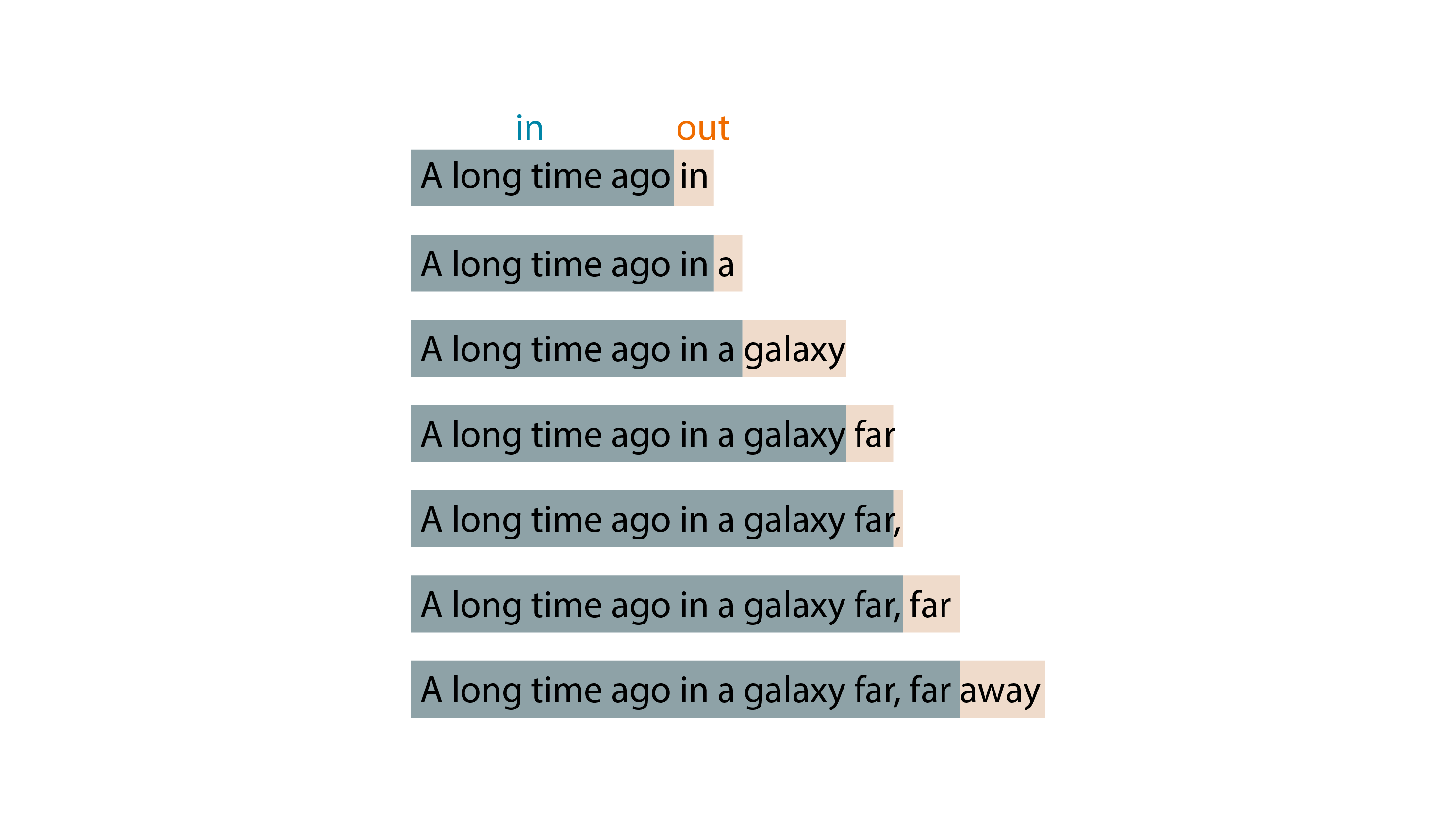
Before we dive into how to construct a GPT model, let’s start by understanding how we’ll invoke it. We’ll assume for the moment that we have a working GPT model, and focus on how to prepare the input, call the model, and interpret the output. The general idea is to provide a few words as input to kick-start the generation, and return text that is likely to follow that input. For example, if we give a GPT model the input “A long time ago”, the model might return as output “in a galaxy far, far away”.

Let’s take a look at the code we’ll use to invoke our model, passing the input “A long time ago” and generating 10 new tokens. I’ve used comments to show the shape of each tensor. I’ll explain more of the details after the code.

import tiktoken

def tokenize(text, batch_size):
    """Convert text to numerical tokens and repeat batch_size times."""
    encoding = tiktoken.encoding_for_model("davinci")
    token_list = encoding.encode(text)
    token_tensor = torch.tensor(token_list, dtype=torch.long) # (input_seq_len)
    token_tensor = token_tensor.unsqueeze(0) # (1, input_seq_len)
    token_tensor = token_tensor.repeat(batch_size, 1) # (batch_size, input_seq_len)
    return encoding, token_tensor

def limit_sequence_length(input_tokens, block_size):
    """Limit the input to at most block_size tokens."""
    input_seq_len = input_tokens.size(1)
    seq_len = min(input_seq_len, block_size)
    block_tokens = input_tokens[:, -seq_len:] # (batch_size, seq_len)
    return block_tokens

def generate_next_token(model, tokens):
    """Use the highest probability from the Transformer model to choose the next token."""
    mask = subsequent_mask(tokens.size(1)) # (1, seq_len, seq_len)
    decoder_output = model.decode(tokens, mask) # (batch_size, seq_len, vocab_size)
    distribution = model.generator(decoder_output[:, -1, :]) # (batch_size, vocab_size)
    next_token = torch.argmax(distribution, dim=1, keepdim=True) # (batch_size, 1)
    return next_token

# Define constants.
input_text = "A long time ago"
new_token_count = 10
batch_size = 1
block_size = 1024

# Tokenize the input text.
encoding, tokens = tokenize(input_text, batch_size)

# Create the model.
model = make_model(encoding.n_vocab)

# Iterate until we've generated enough new tokens.
for _ in range(new_token_count):
    block_tokens = limit_sequence_length(tokens, block_size) # (batch_size, seq_len)
    next_token = generate_next_token(model, block_tokens) # (batch_size, 1)
    tokens = torch.cat([tokens, next_token], dim=1) # (batch_size, input_seq_len + 1)

# Print each of the generated token sequences.
print(tokens)
for row in tokens:
    print(encoding.decode(row.tolist()))

Since we begin with the string “A long time ago”, you might be inclined to think that a Transformer receives a string as input. However, just like other neural networks, a Transformer requires numerical inputs, so the input string must first be converted into a sequence of numbers. We do that conversion in the tokenize function using a tokenizer (tiktoken from OpenAI, in our example), which breaks up the text into chunks of a few letters, and assigns a number called a token to each unique chunk. To get the correct input for our Transformer, we place the sequence of tokens in a tensor and expand it to include a batch dimension. That’s because, just like other types of neural networks, a Transformer can be trained most efficiently by using batches to take advantage of parallel computations on GPUs. Our example code is running inference on one sequence, so our batch_size is one, but you can experiment with larger numbers if you want to generate multiple sequences at once.

After we’ve tokenized our input, we create the Transformer model using the make_model function, which we’ll discuss later in detail. You might think that invoking the model would return several tokens as output, since this is the typical text generation scenario. However, the Transformer is only able to generate a single token each time it’s called. Since we want to generate many tokens, we use a for loop to call it multiple times, and in each iteration we append the newly generated token to the original sequence of tokens using torch.cat.

GPT-style Transformer models typically have a well-defined token limit: for example, gpt-35-turbo (Chat GPT) has a limit of 4096 tokens, and gpt-4-32k has a limit of 32768 tokens. Since we pass to the Transformer model the concatenation of the input tokens and all output tokens generated so far, the token limit of the model refers to the total number of input plus output tokens. In our code, we define this token limit using the block_size constant, and deal with longer sequences of tokens by simply truncating them to the maximum supported length in the limit_sequence_length function.

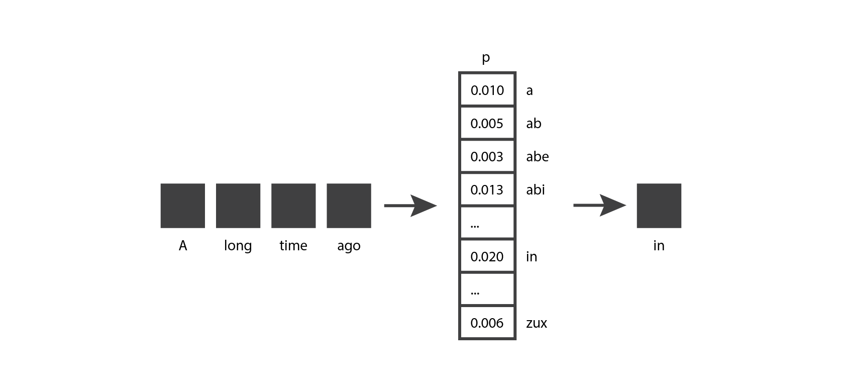
We invoke the Transformer model in the generate_next_token function by calling model.decode followed by model.generator, which correspond to the two major sections of the Transformer architecture. The decoding section expects a mask, which we create using the subsequent_mask function. We’ll analyze all of these functions in detail later in this article. The generation phase returns a sequence of probability distributions, and we select the last one (we’ll see why later), which we use to predict the next token. This distribution contain a probability value for each possible token, representing how likely it is for that token to come next in the sentence.

To make our example code simple and readable, we choose the token that has the highest probability in the output distribution (using torch.argmax). In actual GPT models, the next token is chosen by sampling from the probability distribution, which introduces some variability in the output that makes the text feel more natural. If you have access to the “Completions playground” in the Azure AI Studio, you may have noticed the “Temperature” and “Top probabilities” sliders, which give you some control over how this sampling is done.

If you run this code, you’ll see that the generated output is nonsense. This is completely expected, since we haven’t trained the model and it was initialized with random weights.

tensor([[   32,   890,   640,  2084,  3556, 48241, 26430, 34350, 28146, 43264,
          3556,  6787, 45859, 13884]])
A long time ago</ spaghetti Rapiddx Rav unresolved</ rail MUCHkeeper

In this article we’ll be focusing on the code for the Transformer model architecture, rather than the code for training the model, since that’s where we’ll find the bulk of the Transformer’s innovations. I’ll give you some pointers to train the model at the end, in case you’re interested in extending this code to generate better results.

We now have a good understanding of the inputs and outputs of our Transformer model, and how we instantiate and invoke it. Next we’ll delve into the implementation details of the model itself.

Overview of Transformer architecture

Let’s get familiar with the high-level architecture of the GPT transformer:

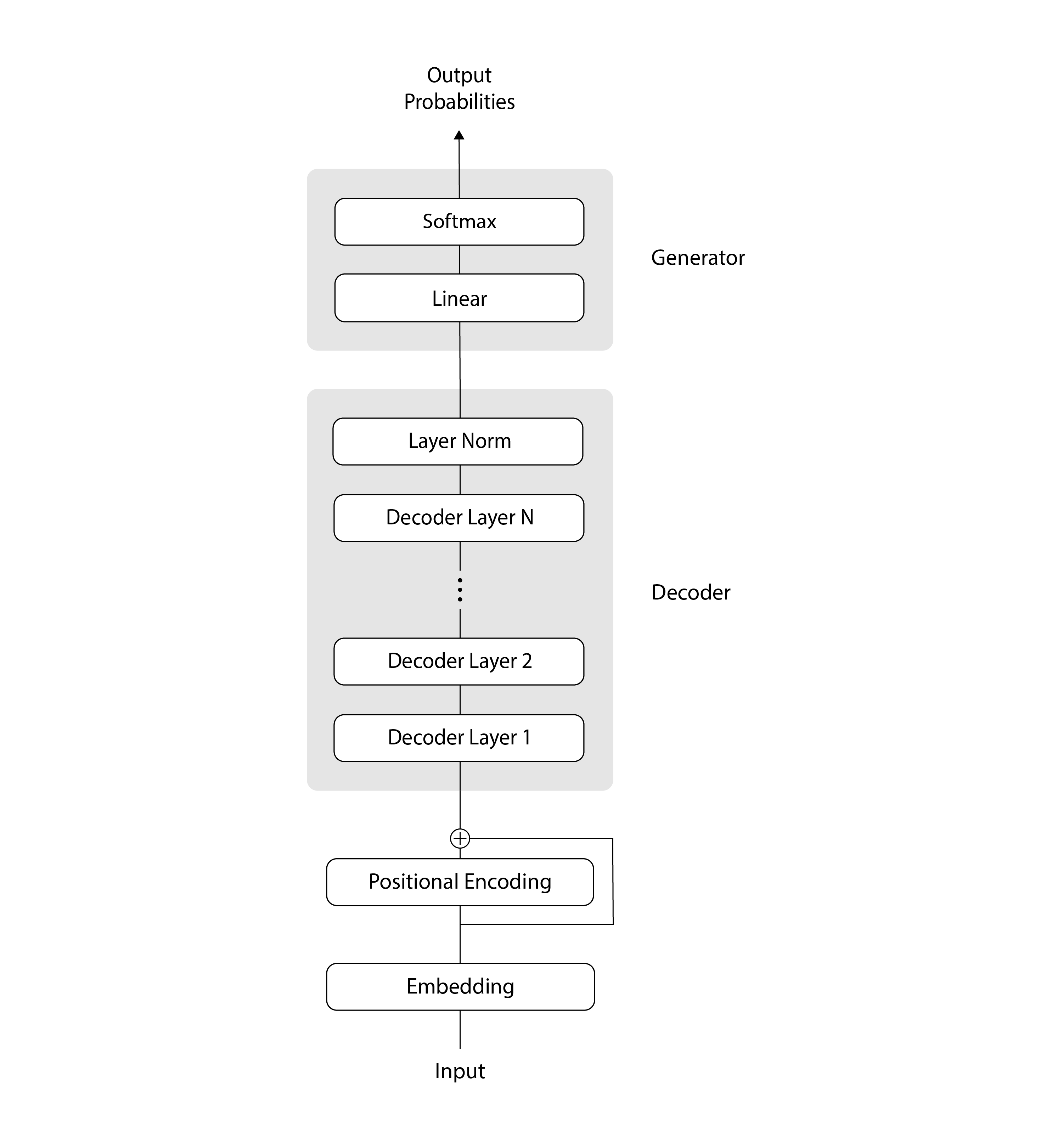
In this diagram, the data flows from the bottom to the top, as is traditional in Transformer illustrations. Initially, our input tokens undergo a couple of encoding steps: they’re encoded using an Embedding layer, followed by a Positional Encoding layer, and then the two encodings are added together. Next, our encoded inputs go through a sequence of N decoding steps, followed by a normalization layer. And finally, we send our decoded data through a linear layer and a softmax, ending up with a probability distribution that we can use to select the next token.

In the sections that follow, we’ll take a closer look at each of the components in this architecture.

Embedding

The Embedding layer turns each token in the input sequence into a vector of length d_model. The input of the Transformer consists of batches of sequences of tokens, and has shape (batch_size, seq_len). The Embedding layer takes each token, which is a single number, calculates its embedding, which is a sequence of numbers of length d_model, and returns a tensor containing each embedding in place of the corresponding original token. Therefore, the output of this layer has shape (batch_size, seq_len, d_model).

import torch.nn as nn

class Embeddings(nn.Module):

    def __init__(self, d_model, vocab_size):
        super(Embeddings, self).__init__()
        self.lut = nn.Embedding(vocab_size, d_model)
        self.d_model = d_model

    # input x: (batch_size, seq_len)
    # output: (batch_size, seq_len, d_model)
    def forward(self, x):
        out =  self.lut(x) * math.sqrt(self.d_model)
        return out

The purpose of using an embedding instead of the original token is to ensure that we have a similar mathematical vector representation for tokens that are semantically similar. For example, let’s consider the words “she” and “her”. These words are semantically similar, in the sense that they both refer to a woman or girl, but the corresponding tokens can be completely different (for example, when using OpenAI’s tiktoken tokenizer, “she” corresponds to token 7091, and “her” corresponds to token 372). The embeddings for these two tokens will start out being very different from one another as well, because the weights of the embedding layer are initialized randomly and learned during training. But if the two words frequently appear nearby in the training data, eventually the embedding representations will converge to be similar.

Positional Encoding

The Positional Encoding layer adds information about the absolute position and relative distance of each token in the sequence. Unlike recurrent neural networks (RNNs) or convolutional neural networks (CNNs), Transformers don’t inherently possess any notion of where in the sequence each token appears. Therefore, to capture the order of tokens in the sequence, Transformers rely on a Positional Encoding.

There are many ways to encode the positions of tokens. For example, we could implement the Positional Encoding layer by using another embedding module (similar to the previous layer), if we pass the position of each token rather than the value of each token as input. Once again, we would start with the weights in this embedding chosen randomly. Then during the training phase, the weights would learn to capture the position of each token.

The authors of The Annotated Transformer code decided to implement a more sophisticated algorithm that precomputes a representation for the positions of tokens in the sequence. Since we want to follow their code as closely as possible, we’ll use the same approach:

class PositionalEncoding(nn.Module):

    def __init__(self, d_model, dropout, max_len=5000):
        super(PositionalEncoding, self).__init__()
        self.dropout = nn.Dropout(p=dropout)

        pe = torch.zeros(max_len, d_model)
        position = torch.arange(0, max_len).unsqueeze(1)  # (max_len, 1)
        div_term = torch.exp(
            torch.arange(0, d_model, 2) *
            -(math.log(10000.0) / d_model))  # (d_model/2)

        pe[:, 0::2] = torch.sin(position * div_term)  # (max_len, d_model)
        pe[:, 1::2] = torch.cos(position * div_term)  # (max_len, d_model)
        pe = pe.unsqueeze(0)  # (1, max_len, d_model)
        self.register_buffer('pe', pe)

    # input x: (batch_size, seq_len, d_model)
    # output: (batch_size, seq_len, d_model)
    def forward(self, x):
        x = x + Variable(self.pe[:, :x.size(1)], requires_grad=False)
        return self.dropout(x)

This positional encoding uses sines and cosines of varying frequencies to populate a pe tensor. For example, in the illustration below, the values in blue and red were calculated using sine waves of two different frequencies, and the values in orange and green were calculated using cosine waves of those same frequencies.

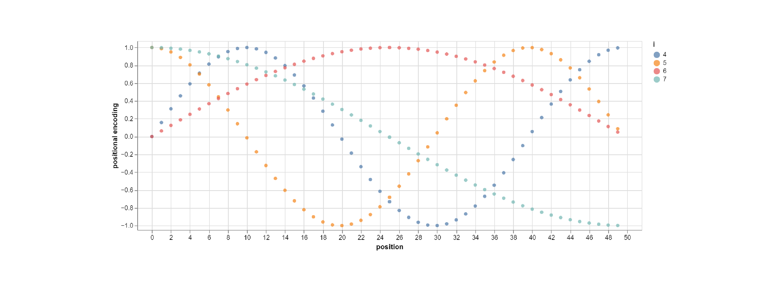
The values of the sine and cosine graphs end up populating the columns of the pe tensor, as shown below:

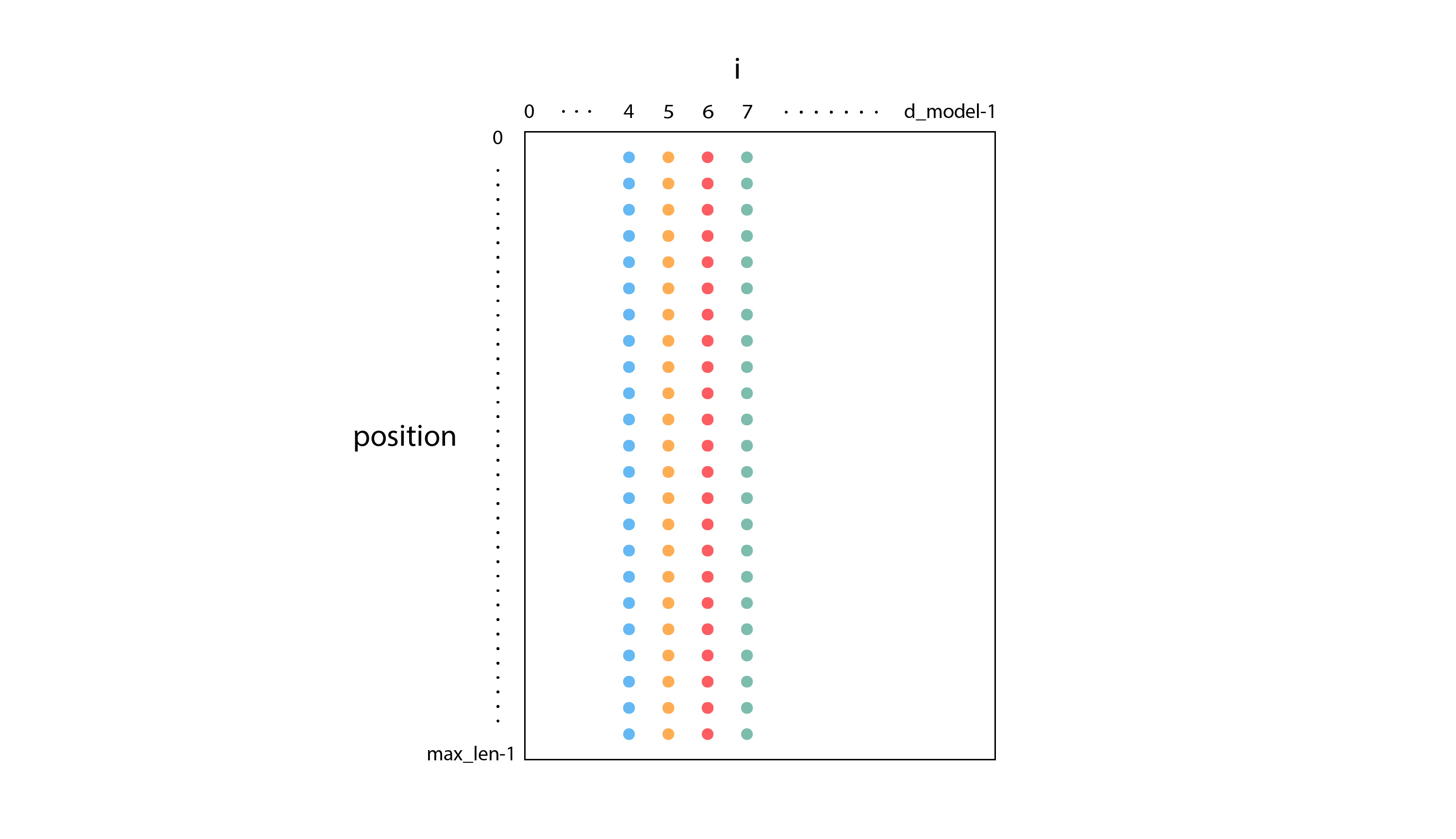
Then during the “forward” phase, we receive the result x of the previous Embedding layer as input, and we return the sum of x and pe.

The main advantage of precomputing the values for the positional encoding (rather than using a trainable Embedding) is that our model ends up with fewer parameters to train. This reduction in parameters leads to improved training performance, which is tremendously important when working with large language models.

Decoder

As we saw in the diagrammatic overview of the Transformer architecture, the next stage after the Embedding and Positional Encoding layers is the Decoder module. The Decoder consists of N copies of a Decoder Layer followed by a Layer Norm. Here’s the Decoder class, which takes a single DecoderLayer instance as input to the class initializer:

class Decoder(nn.Module):

    def __init__(self, layer, N):
        super(Decoder, self).__init__()
        self.layers = clones(layer, N)
        self.norm = LayerNorm(layer.size)

    def forward(self, x, mask):
        for layer in self.layers:
            x = layer(x, mask)
        return self.norm(x)

The clones function simply creates a PyTorch list containing N copies of a module:

def clones(module, N):
    return nn.ModuleList([copy.deepcopy(module) for _ in range(N)])

The Layer Norm takes an input of shape (batch_size, seq_len, d_model) and normalizes it over its last dimension. As a result of this step, each embedding distribution will start out as unit normal (centered around zero and with standard deviation of one). Then during training, the distribution will change shape as the parameters a_2 and b_2 are optimized for our scenario. You can learn more about Layer Norm in the Layer Normalization paper from 2016.

class LayerNorm(nn.Module):

    def __init__(self, features, eps=1e-6):
        super(LayerNorm, self).__init__()
        self.a_2 = nn.Parameter(torch.ones(features))
        self.b_2 = nn.Parameter(torch.zeros(features))
        self.eps = eps

    def forward(self, x):
        mean = x.mean(-1, keepdim=True)
        std = x.std(-1, keepdim=True)
        return self.a_2 * (x - mean) / (std + self.eps) + self.b_2

The DecoderLayer class that we clone has the following architecture:

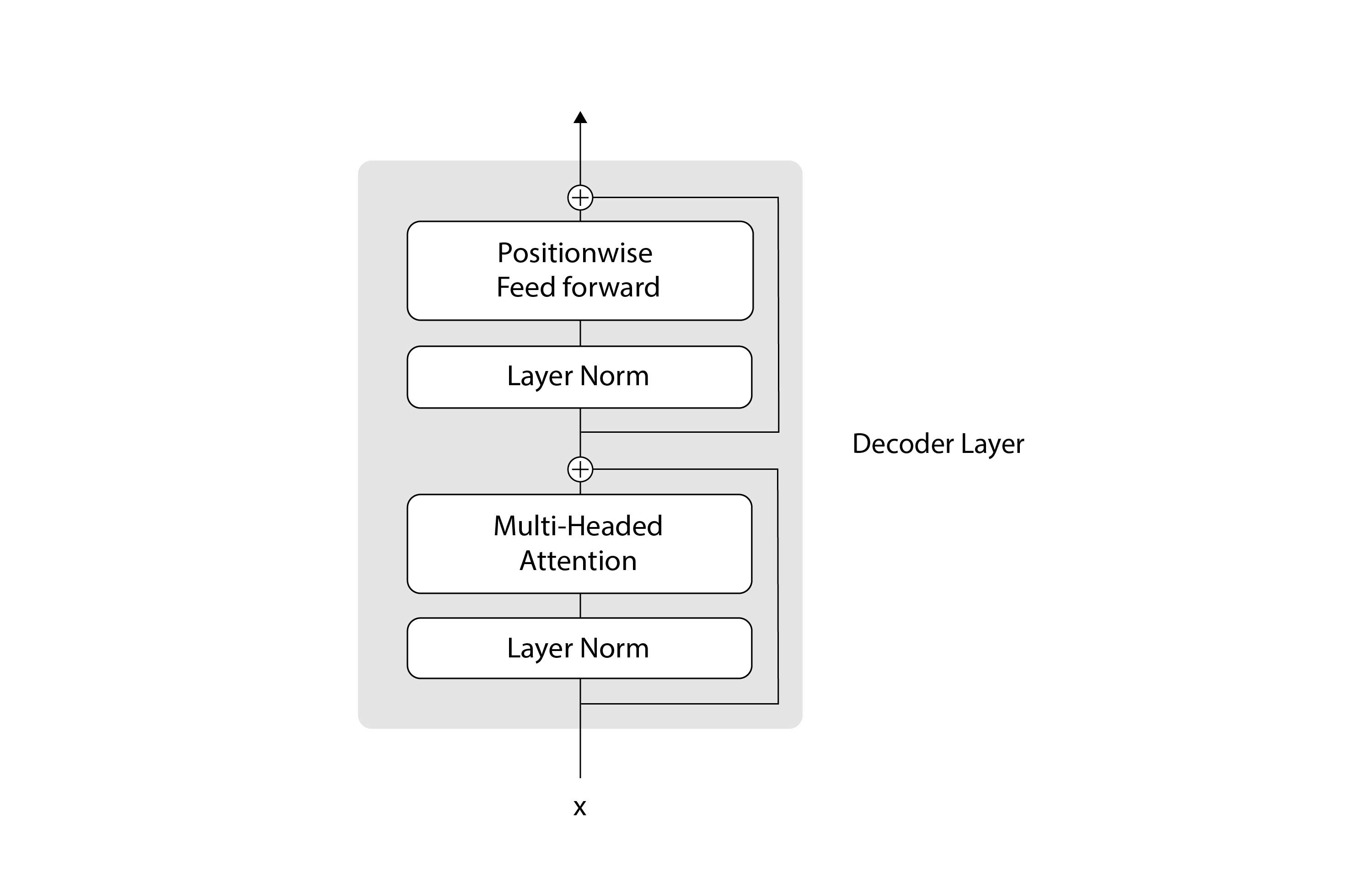
Here’s the corresponding code:

class DecoderLayer(nn.Module):

    def __init__(self, size, self_attn, feed_forward, dropout):
        super(DecoderLayer, self).__init__()
        self.size = size
        self.self_attn = self_attn
        self.feed_forward = feed_forward
        self.sublayer = clones(SublayerConnection(size, dropout), 2)

    def forward(self, x, mask):
        x = self.sublayer[0](x, lambda x: self.self_attn(x, x, x, mask))
        return self.sublayer[1](x, self.feed_forward)

At a high level, a DecoderLayer consists of two main steps: the attention step, which is responsible for the communication between tokens, and the feed forward step, which is responsible for the computation of the predicted tokens. Surrounding each of those steps, we have residual (or skip) connections, which are represented by the plus signs in the diagram. Residual connections provide an alternative path for the data to flow in the neural network, which allows skipping some layers. The data can flow through the layers within the residual connection, or it can go directly through the residual connection and skip the layers within it. In practice, residual connections are often used with deep neural networks, because they help the training to converge better. You can learn more about residual connections in the paper Deep residual learning for image recognition, from 2015. We implement these residual connections using the SublayerConnection module:

class SublayerConnection(nn.Module):

    def __init__(self, size, dropout):
        super(SublayerConnection, self).__init__()
        self.norm = LayerNorm(size)
        self.dropout = nn.Dropout(dropout)

    def forward(self, x, sublayer):
        return x + self.dropout(sublayer(self.norm(x)))

The feed-forward step is implemented using two linear layers with a Rectified Linear Unit (ReLU) activation function in between:

class PositionwiseFeedForward(nn.Module):

    def __init__(self, d_model, d_ff, dropout=0.1):
        super(PositionwiseFeedForward, self).__init__()
        self.w_1 = nn.Linear(d_model, d_ff)
        self.w_2 = nn.Linear(d_ff, d_model)
        self.dropout = nn.Dropout(dropout)

    def forward(self, x):
        return self.w_2(self.dropout(F.relu(self.w_1(x))))

The attention step is the most important part of the Transformer, so we’ll devote the next section to it.

Masked multi-headed self-attention

The multi-headed attention section in the previous diagram can be expanded into the following architecture:

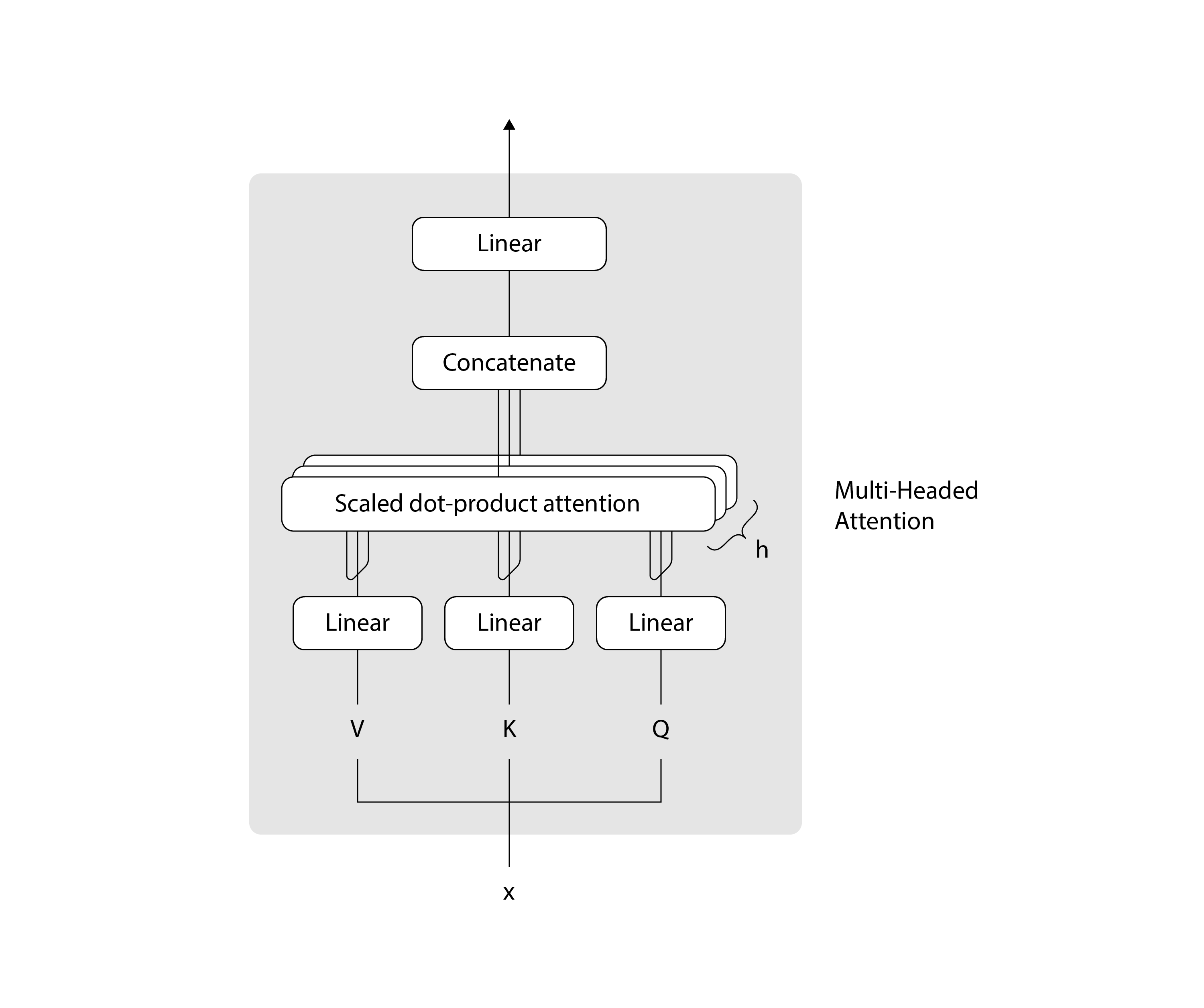
As the name implies, the multi-headed attention module processes several instances of attention computations in parallel, with some additional pre- and post-processing of the data.

class MultiHeadedAttention(nn.Module):

    def __init__(self, h, d_model, dropout=0.1):
        super(MultiHeadedAttention, self).__init__()
        assert d_model % h == 0
        self.d_k = d_model // h
        self.h = h
        self.linears = clones(nn.Linear(d_model, d_model), 4)
        self.attn = None
        self.dropout = nn.Dropout(p=dropout)

    def forward(self, query, key, value, mask=None):
        if mask is not None:
            mask = mask.unsqueeze(1)  # (1, 1, seq_len, seq_len)

        nbatches = query.size(0)  # batch_size

        # (batch_size, seq_len, d_model) => (batch_size, h, seq_len, d_k)
        query, key, value = \
            [l(x).view(nbatches, -1, self.h, self.d_k).transpose(1, 2)
             for l, x in zip(self.linears, (query, key, value))]

        # (batch_size, h, seq_len, d_k)
        x, self.attn = attention(query,
                                 key,
                                 value,
                                 mask=mask,
                                 dropout=self.dropout)

        # (batch_size, h, seq_len, d_k) => (batch_size, seq_len, d_model)
        x = x.transpose(1, 2).contiguous().view(nbatches, -1, self.h * self.d_k)
        return self.linears[-1](x)

The inputs to the multi-headed attention layer include three tensors called query (), key (), and value (). In our particular model, we pass the same tensor for all three of these parameters: the output x of the previous layer, which has shape (batch_size, seq_len, d_model) (this is why we call it self-attention). We pre-process these three tensors by first passing each through a linear layer, then splitting them into h attention heads of size d_k where h * d_k = d_model, resulting in tensors of shape (batch_size, seq_len, h, d_k). Then we transpose dimensions 1 and 2 to produce tensors of shape (batch_size, h, seq_len, d_k). Next we compute attention for each head, resulting in tensors of the same shape. And finally, our post-processing concatenates all the heads back into tensors of shape (batch_size, seq_len, d_model), and passes them through one more linear layer. By using tensor operations to do all the attention computations in each head in parallel, we can take full advantage of the GPU.

Attention is calculated using the following formula:

Here’s the code that implements the formula:

# Dimensions of query, key, and value: (batch_size, h, seq_len, d_k)
# Dimensions of mask: (1, 1, seq_len, seq_len)
def attention(query, key, value, mask=None, dropout=None):
    d_k = query.size(-1)
    # (batch_size, h, seq_len, d_k) x (batch_size, h, d_k, seq_len) -> (batch_size, h, seq_len, seq_len)
    scores = torch.matmul(query, key.transpose(-2, -1)) / math.sqrt(d_k)
    if mask is not None:
        scores = scores.masked_fill(mask == 0, -1e9)
    p_attn = F.softmax(scores, dim=-1) # (batch_size, h, seq_len, seq_len)
    if dropout is not None:
        p_attn = dropout(p_attn)
    # (batch_size, h, seq_len, seq_len) x (batch_size, h, seq_len, d_k) -> (batch_size, h, seq_len, d_k)
    return torch.matmul(p_attn, value), p_attn 

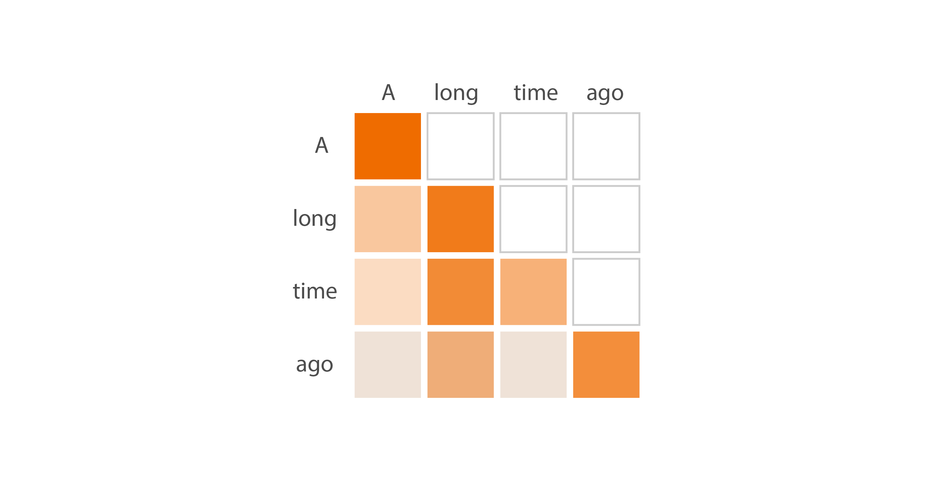
At a high level, the attention algorithm determines which tokens in the input sequence it should pay more attention to, and then uses that information to predict the next token. In the image below, darker shades of orange represent tokens that are more relevant in the prediction.

More specifically, attention actually predicts the next token for several portions of our input sequence. It looks at the first token and predicts what a second token might be, then it looks at the first and second tokens and predicts what a third token might be, and so on.

This seems a bit wasteful during inference because we’re only interested in the last prediction. However, this is extremely useful during training. If you give the Transformer n tokens as input, it will be trained to receive inputs of lengths from 1 to n-1, so the model is better able to handle inputs of different lengths in the future.

The idea in the diagram above is represented by the p_attn tensor in the code. This tensor has shape (batch_size, h, seq_len, seq_len), but let’s ignore the batch size and number of heads for now (each batch and each head work identically), and consider just one tensor slice of shape (seq_len, seq_len). Each row in the p_attn tensor contains a probability distribution, indicating how interesting all other key tokens are to the query token corresponding to that row. The resulting tensor encapsulates all the values shown in the previous image:

You can see in the code exactly how this tensor is calculated. We first do a matrix multiplication between the query and the transposed key. If we ignore the batch size and number of heads, the query and key consist of a sequence of embeddings of shape (seq_len, d_k), which are the result of sending the input x through different linear layers. When we multiply the query tensor of shape (seq_len, d_k) with the transposed key tensor of shape (d_k, seq_len), we’re essentially doing a dot-product between each embedding in the query and all other embeddings in the key, ending up with a tensor scores of shape (seq_len, seq_len). A large value of the dot product indicates that a particular embedding in the query has “taken an interest” in a particular embedding in the key, or in other words, the model has discovered an affinity between two positions in the input sequence. Roughly speaking, we now have a tensor that represents how “interesting” or “important” each token finds all other tokens in the sequence.

The next step is to apply a mask to the scores tensor that causes the values in its upper triangle to be ignored (which is why we call it masked attention). We do this because in the GPT-style text generation scenario, the model looks only at past tokens when predicting the next token. We use the following code to define a mask that contains the value True in its diagonal and lower triangle, and False in its upper triangle:

def subsequent_mask(size):
    """
    Mask out subsequent positions.
    """
    attn_shape = (1, size, size)
    subsequent_mask = torch.triu(torch.ones(attn_shape),
                                 diagonal=1).type(torch.uint8)
    return subsequent_mask == 0

We apply this mask to the scores tensor using the masked_fill function, replacing all the values in the upper-triangle with a negative number of very large magnitude.

Last, we apply a softmax that converts each row in the tensor into a probability distribution. Remember the formula for softmax?

Since raised to a negative power of very large magnitude is close to zero, all the values in the upper-triangle of the p_attn tensor essentially become zero. The remaining values (in the lower triangle and diagonal) become probabilities that sum to one in each row.

You may have noticed that in the code, when we multiplied the query and key tensors, we divided all the values in the resulting matrix by the square root of d_k. We did that to keep the variance close to one, which ensures that the softmax gives us probability values that are well distributed along the whole range, from zero to one. If we hadn’t done that, the distributions calculated by softmax could approach one-hot vectors, where one value is one and the others are all zero — which would make the output of the model seem predictable and robotic.

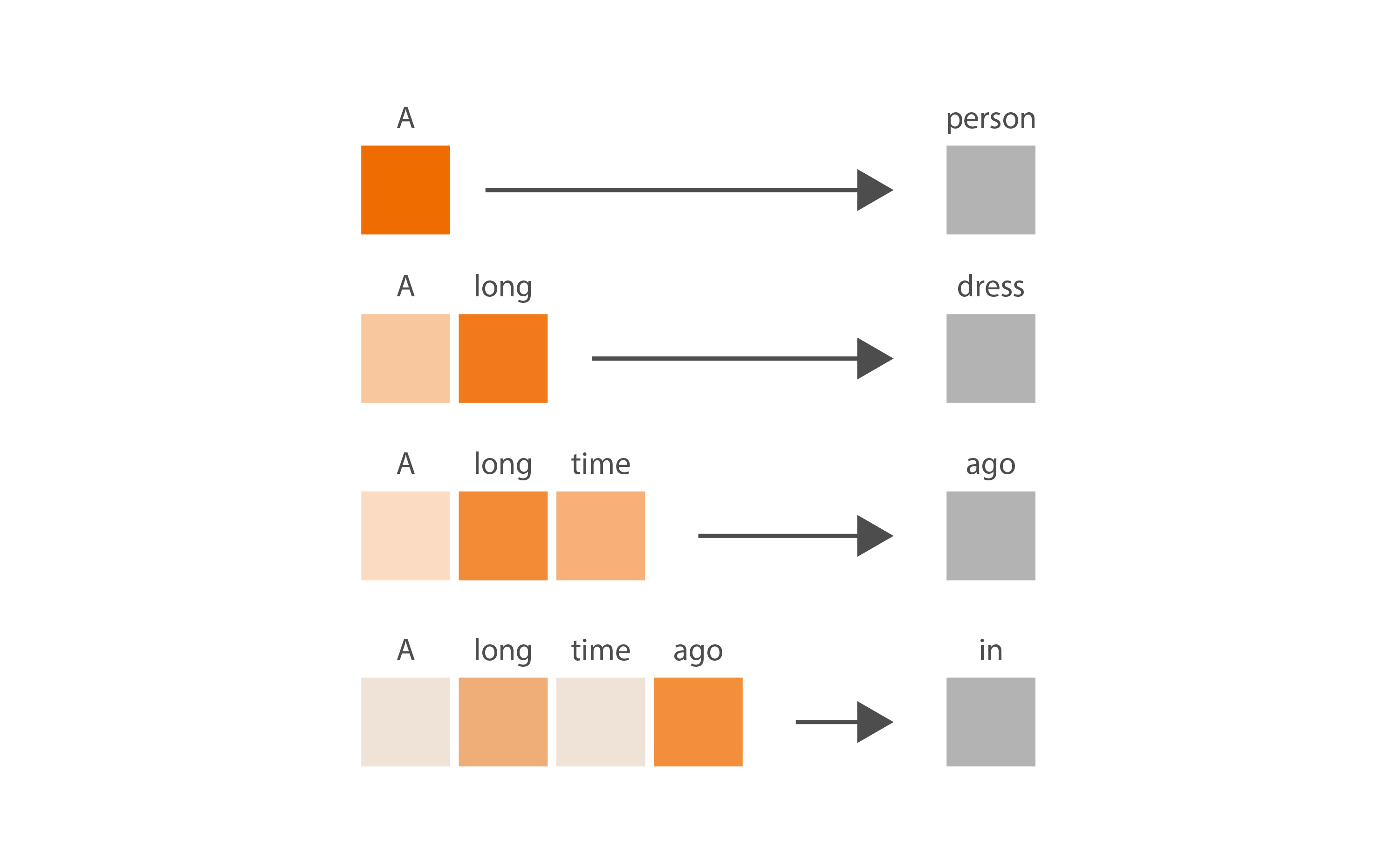
At this point, we have a p_attn tensor containing probability distributions along its rows, representing how interesting tokens are to each other. The next step is to use this measure of interest to determine how much attention we should pay to each input token, while generating the output token. Naturally, we’ll pay more attention to the most interesting tokens. We generate the next token by multiplying our tensor of probabilities by our value tensor, which contains the input token embeddings x after applying a linear layer. The resulting tensor will contain a prediction for each token subsequence:

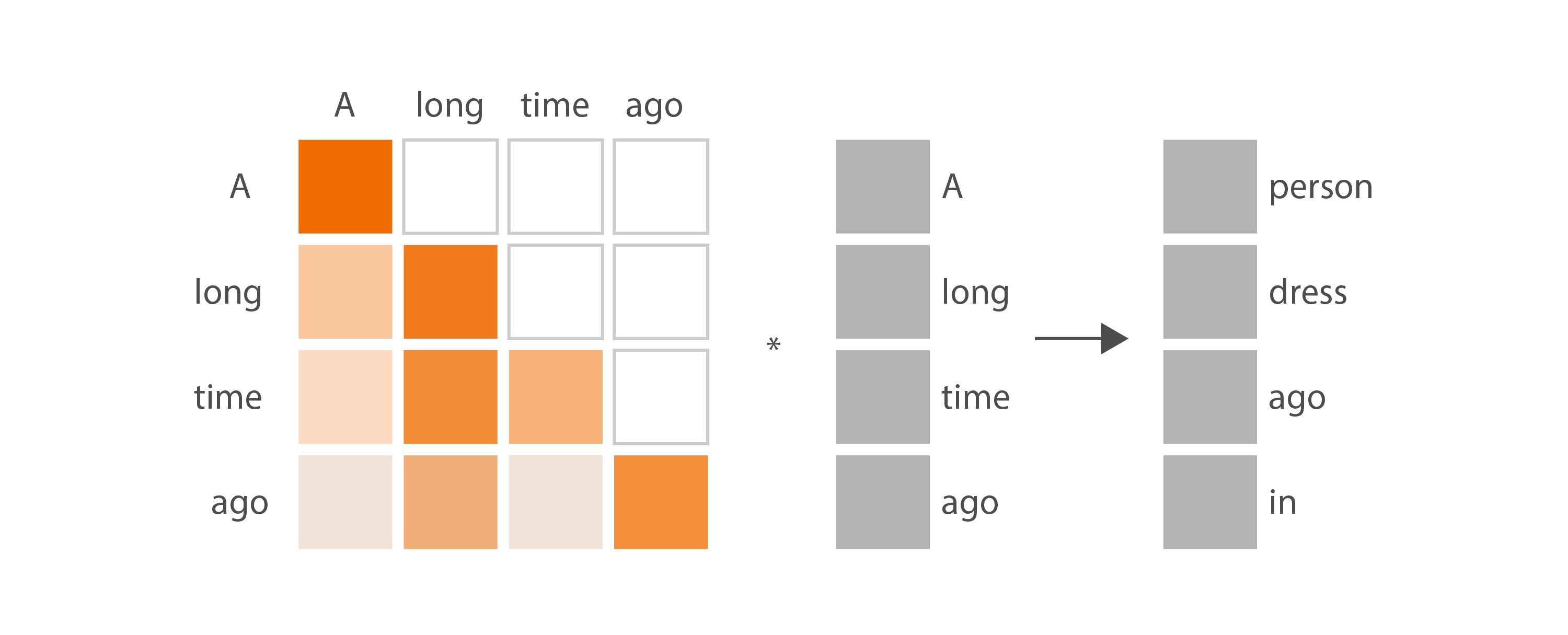
Here’s the intuition for this diagram: for the input subsequence “A”, we pay full attention to the one and only input token, and might produce a next-token prediction such as “person”. For the input subsequence “A long”, our model has been trained to pay a bit more attention to the token “long” than to the token “A”, and might produce the next-token prediction “dress”. And so on. When doing inference we want to take into account the full input sequence “A long time ago”, so we only care about the last row in this diagram. We pay most attention to “ago”, we pay a little less attention to “long”, we pay the least attention to the other two tokens, and we produce a next-token prediction of “in”.

After we’ve calculated attention for all the heads, and have concatenated the results back together, we have an output tensor of dimension (batch_size, seq_len, d_model). This tensor contains the token predictions for each sub-sequence, and is almost ready to be returned to the user. But before we do that, we need one last step to finalize its shape and contents.

Generator

The last step in our Transformer is the Generator, which consists of a linear layer and a softmax executed in sequence:

class Generator(nn.Module):

    def __init__(self, d_model, vocab):
        super(Generator, self).__init__()
        self.proj = nn.Linear(d_model, vocab)

    def forward(self, x):
        return F.log_softmax(self.proj(x), dim=-1)

The purpose of the linear layer is to convert the third dimension of our tensor from the internal-only d_model embedding dimension to the vocab_size dimension, which is understood by the code that calls our Transformer. The result is a tensor dimension of (batch_size, seq_len, vocab_size). The purpose of the softmax is to convert the values in the third tensor dimension into a probability distribution. This tensor of probability distributions is what we return to the user.

You might remember that at the very beginning of this article, we explained that the input to the Transformer consists of batches of sequences of tokens, of shape (batch_size, seq_len). And now we know that the output of the Transformer consists of batches of sequences of probability distributions, of shape (batch_size, seq_len, vocab_size). Each batch contains a distribution that predicts the token that follows the first input token, another distribution that predicts the token that follows the first and second input tokens, and so on. The very last probability distribution of each batch enables us to predict the token that follows the whole input sequence, which is what we care about when doing inference.

The Generator is the last piece of our Transformer architecture, so we’re ready to put it all together.

Putting it all together

We use the DecoderModel module to encapsulate the three main pieces of the Transformer architecture: the embeddings, the decoder, and the generator.

class DecoderModel(nn.Module):

    def __init__(self, decoder, embed, generator):
        super(DecoderModel, self).__init__()
        self.embed = embed
        self.decoder = decoder
        self.generator = generator

    def forward(self, x, mask):
        return self.decode(x, mask)

    def decode(self, x, mask):
        return self.decoder(self.embed(x), mask)

Calling decode executes just the embeddings and decoder, so if we want to execute all steps of the Transformer, we need to call decode followed by generator. That’s exactly what we did in the generate_next_token function of the inference code that I showed at the beginning of this post.

The inference code also calls a make_model function that returns an instance of DecoderModel. This function initializes all the components we’ve discussed so far, and puts them together according to the architecture diagram at the beginning of this post:

def make_model(vocab_size, N=6, d_model=512, d_ff=2048, h=8, dropout=0.1):
    c = copy.deepcopy
    attn = MultiHeadedAttention(h, d_model)
    ff = PositionwiseFeedForward(d_model, d_ff, dropout)
    position = PositionalEncoding(d_model, dropout)
    model = DecoderModel(
        Decoder(DecoderLayer(d_model, c(attn), c(ff), dropout), N),
        nn.Sequential(Embeddings(d_model, vocab_size), c(position)),
        Generator(d_model, vocab_size))

    for p in model.parameters():
        if p.dim() > 1:
            nn.init.xavier_uniform_(p)
    return model

We now have all the pieces needed to implement a GPT-style Transformer architecture!

We’ll finish with a few thoughts on training, and we’ll do a brief comparison between the full Transformer and the GPT-style subset.

Training

The code for training the GPT-style Transformer is the same as the code for training any other neural network — except that in our scenario, for each input sequence of tokens, we expect the output to be the sequence that begins one position to the right. For example, if we give it “A long time ago” as input, we expect the sampling of the probabilities returned by the model to produce “long time ago in”.

If you have experience training neural networks and want to train the Transformer on your own, you can reuse any code you’ve written in the past and adapt it to our scenario. If you need guidance, I recommend that you follow the code and explanations in Part 2 of the Annotated Transformer. Either way, you’ll need access to a fast GPU, locally or in the cloud. I’m partial to training in the cloud on Azure of course!

Comparison with full Transformer

Once you understand the architecture of the GPT-style Transformer, you’re a short step away from understanding the full Transformer as it’s presented in the Attention is all you need paper. Below you can see the diagram of the Transformer architecture presented in the paper, with the parts we covered in this post enclosed by an orange box.

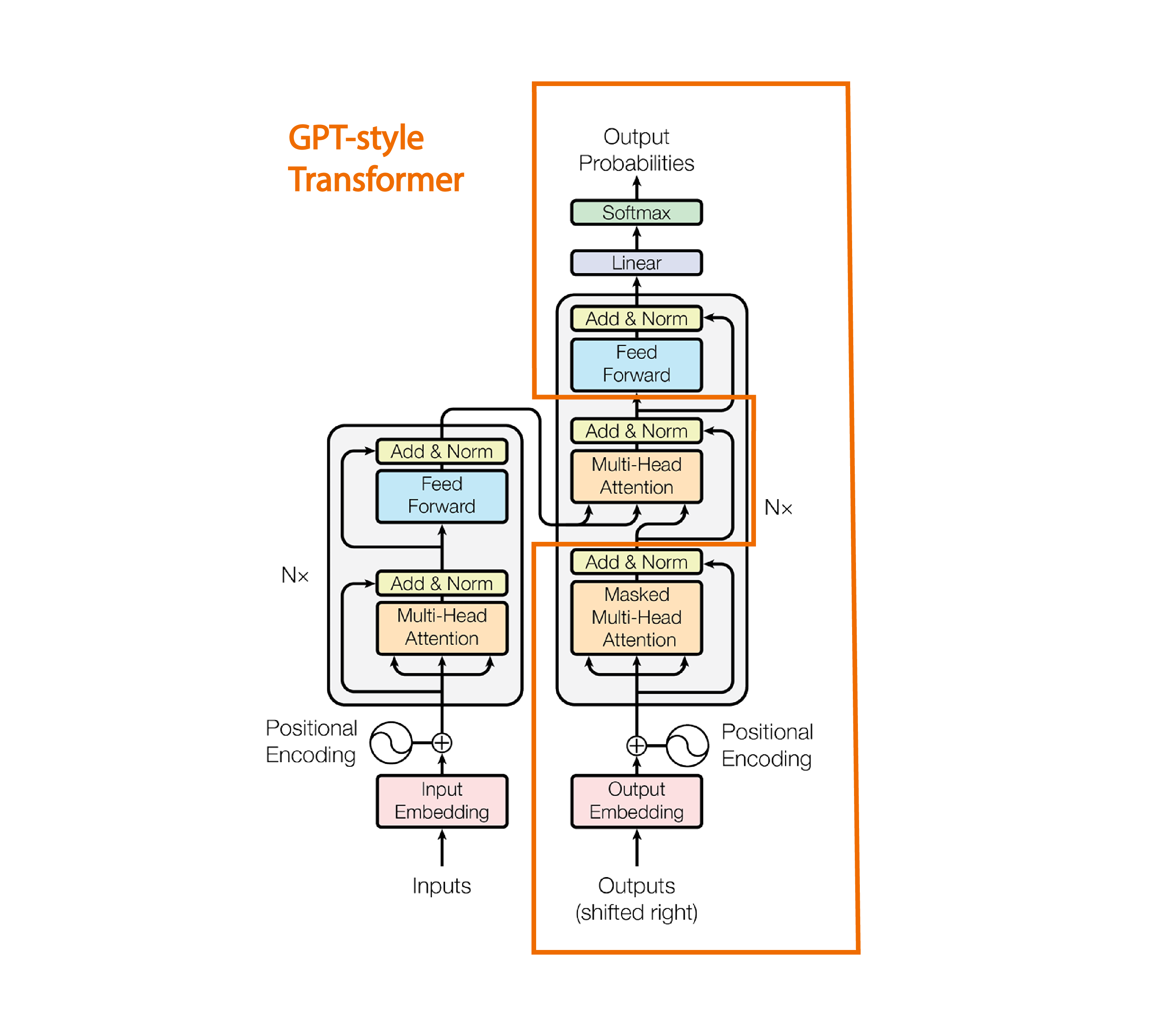
Illustration adapted from the Attention is all you need paper

The full Transformer has an encoder section (on the left) and a decoder section (on the right). The original intent of the paper was to present an architecture for machine translation. In that context, the encoder was used to process the input language, and the decoder was used to produce the output language.

You can see that in addition to the masked multi-headed self-attention used in the GPT-style Transformer, the full Transformer has two other multi-headed attention blocks. The one in the encoder is not masked, which means that the p_attn tensor we saw in the attention section doesn’t have the values in its upper-triangular section zeroed out. That’s because in machine translation, generating a single output language token may require the model to pay attention to input language tokens in all sequence positions, including earlier and later positions. The additional multi-headed attention block in the decoder section is a “cross-attention” (as opposed to “self-attention”) layer which means that its key and value come from a different source than the query, as you can see in the diagram. That’s because the model needs to understand how much attention it should pay to each token in the input language, as it predicts tokens in the output language. The rest of the pieces of the diagram are similar to parts of the GPT-style Transformer, and have already been explained in this post.

Conclusion

In this article, we discussed the architecture of a GPT-style Transformer model in detail, and covered the architecture of the original Transformer at a high level. Given the increasing popularity of GPT models in the industry, and how often variations of the original Transformer model come up in recent papers, I hope that you’ll find this knowledge useful in your job or education. If you want to go deeper, I encourage you to clone the associated GitHub project and explore the code. Set breakpoints in any section of the code that isn’t clear to you, run it, and inspect its variables. If you have access to a GPU, write code that trains it and see the performance of its predictions improve.

With your newly acquired knowledge, I hope that you can help the AI community demystify some of the misconceptions associated with these models. Many people in the general public assume that these models have a higher-level understanding of the world, which you now know is not the case. They’re simply composed of mathematical and statistical operations aimed at predicting the next token based on previous training data. Maybe future versions of generative models will have a better understanding of the world, and generate even better predictions? If so, I’ll be here to tell you all about it.

Note

All images are by the author unless otherwise noted. You can use any of the original images in this blog post for any purpose, with attribution (a link to this article).